1 Introduction & Overview [M. Visbeck, Chief Scientist]

1.1 AnSlope, the Program

AnSlope's primary goal is to identify the principal physical processes that govern the transfer of shelf-modified dense water into intermediate and deep layers of the adjacent deep ocean. At the same time, we seek to understand the compensatory poleward flow of waters from the oceanic regime. We identify the upper continental slope as the critical gateway for the exchange of shelf and deep ocean waters. Four specific objectives: [A] Determine the ASF mean structure and the principal scales of variability (spatial from ~1 km to ~100 km, and temporal from tidal to seasonal), and estimate the role of the Front on cross-slope exchanges and mixing of adjacent water masses; [B] Determine the influence of slope topography (canyons, proximity to a continental boundary, isobath divergence/convergence) on frontal location and outflow of dense Shelf Water; [C] Establish the role of frontal instabilities, benthic boundary layer transports, tides and other oscillatory processes on cross-slope advection and fluxes; and [D] Assess the effect of diapycnal mixing (shear-driven and double-diffusive), lateral mixing identified through intrusions, and nonlinearities in the equation of state (thermobaricity and cabbeling) on the rate of descent and fate of outflowing, near-freezing Shelf Water.

AnSlope core elements are: moorings; CTD-O₂/ADCP and CTD-mounted Microstructure Profiling System (CMiPS); CFC, oxy-18, tritium/helium tracers; and basic tidal modeling.

In addition to the core AnSlope activities we hosted three ancillary projects during this ANSLOPE II cruise: Phytoplankton Biomass Ancillary Project, Cetacean Ancillary Project and dedicated Sea Ice observations.

The cruise activities of these elements are reported below:

• CTD/LADCP/Tracer

• Moorings

• XBT/XCTD section

• Sea Ice

• Phytoplankton Biomass

• Cetacean, marine mammal and wildlife observations

• Antarctic Scout Research Program

International Collaboration: The Italian CLIMA [Climate Long–term Interaction of the Mass balance of Antarctica ] program in the Ross Sea provides a valuable international enhancement for the AnSlope observational component. Giorgio Budillon and Ellio Paschini, who joined the NBP0402 science team brought with them the latest Italica CTD and mooring G data.

The AnSlope field phase consists of three cruises within 12 to 14 months, with moorings in place throughout the period:

AnSlope 1: February 25 to April 11 2003: deploy the mooring array; thermohaline, oxygen and tracer [CFC, oxy-18, tritium/Helium] stratification, circulation and microstructure at beginning of mooring time series. In addition, water samples for nutrient analyses were collected at 60 selected stations to complement the measurements carried out in the Ross Sea in January and February 2003 by the Italian CLIMA project.

AnSlope 2: February 23 to April 10, 2004: thermohaline and oxygen and (limited) tracer stratification, circulation at time of mooring recovery and redeployment;

AnSlope 3: October 6, 2004 to December 10 2004: thermohaline, oxygen and tracer [CFC, oxy-18, tritium/Helium] stratification, circulation and microstructure;

1.2 AnSlope-2 Personnel

Science Staff

Martin Visbeck	Chief Scientist	LDEO
Andreas Thurnherr	LADCP/CTD/tracer sampling	LDEO
Bruce Huber	LADCP/CTD/tracer sampling	LDEO
Philip Mele	CTD/oxygen	LDEO
Erin Stone	oxygen/CTD/bio	LDEO
Suzanne Rab-Green	CFC/autosal	LDEO
Ellio Paschini	CTD/autosal	CLIMA/ISMAR-CNR
Giorgio Budillon	CTD/salinity-cfc sampling	CLIMA/ Università di Napoli "Parthenope"
Alejandro Orsi	Moorings	TAMU
Jay Simpkins	Moorings	OSU
Kathryn Brooksforce	Moorings	OSU
Fred Martwich	Moorings	NASA-Ames
Brendan Hart	Moorings	OSU
Margaret Knuth	Sea ice	Clarkson Univ
William Lipscomb	Sea ice	Los Alamos Laboratory
Ana Širović	Marine Mammal Acoustics	SIO/MPL
Deb Thiele	Cetacean observations	IWC
Deb Glasgow	Cetacean observations	IWC

CLIMA = Climate Long–term Interaction of the Mass balance of Antarctica (Italy)

LDEO = Lamont-Doherty Earth Observatory

OSU = Oregon State University

TAMU = Texas A&M University

IWC=International Whaling Commission

SIO = Scripps Institution of Oceanography

RPSC Support Staff

Marine Projects Coordinator	Karl Newyear
Marine Technician	Jesse Doren
	Emily Constantine
	Annie Coward
	Josh Spillane
Marine Science Technician	Mo Hodgins
Information Technician	Kevin Bliss
	Paul Huckins
	Suzanne O’Hara
Electronics Technician	Sheldon Blackman
	Jeff Otten
As needed	Brad Range

1.3 AnSlope-2 Accomplishments:

The Chief Scientist's weekly SitReps with those of the Karl Newyear document the activities during the AnSlope 2 cruise. Despite at times harsh weather conditions all cruise objectives were met in a timely manner.

The Track and Station array:

Table 1. in the Appendix describes the 232 CTD/LADCP/Tracer stations. The station array is depicted in Figure 1 of the Appendix.

Preliminary Research Results:

AnSlope-2 cruise activities may be divided into several parts:

Our main two goals were to recover all ANSLOPE moorings and to redeploy a subset of them for a second season as well as to extend the hydrographic surveys obtained during the Anslope 1 cruise.

We recovered 11 of the 12 moorings in record time under favorable ice conditions. One mooring could not be located and must be assumed as lost. We deployed 6 moorings in a with the stronger than expected maximum flow velocities. Alex Orsi’s section below gives more detail on each of the moorings and the position of the new array. We also deployed one mooring, supported by Columbia University funding in the downstream outflow from the Drygalski Trough plume. This mooring site holds a lot of potential to study the long term variability of bottom water production in the Ross Sea sector.

We were able to take 232 CTD casts during the cruise. This is first and foremost a consequence of the superb collaboration between ship’s crew, Raytheon science support and the science party. The objectives of the CTD stations were twofold. We wanted to enhance the data set in the high energy core ANSLOPE region near the Drygalski trough outflow as well as to cover the regional scale differences between the Drygalski trough and the other two main sources of new bottom water to the east: The Joides plume and the Glomar Challenger (or Pennell trough) outflow. The latter is also actively studied by a mooring array as part of the Italian CLIMA program.

During this cruise we have taken most CTD stations in section form. Thus we traversed the shelf break front and its associated flow bands on a perpendicular track and choose dense sampling when the bathymetry was rapidly changing.

Of the 33 primary sections taken during the Anslope 2 cruise 24 crossed the shelf break or other mayor ridges while 7 sections were following roughly the shallowest parts of the troughs in order to document the types of water that make up the downslope plumes. We also learned about to on shelf flow of modified Circumpolar Deep Water.

The large scale picture:

After leaving McMurdo and taking several CTD stations in McMurdo sound we passed near the Terra Nova Bay polynya, a year round largely ice free area in the western Ross Sea. Catabatic winds flowing down the cold continental valleys are causing a large loss of heat from the ocean to the atmosphere and thin new ice is formed. As sea water freezes some of the salt is melting out of the ice and this salty brine causes sinks in narrow plumes to the bottom and in the source for the very dense high salinity shelf water. The strong winds blow much of the new ice out of the bay and thus allow for more new ice production and salty brine release. Terra Nova Bay is believed to be the primary source for Ross Sea high salinity shelf water.

Our first section followed the axis of the Drygalski trough from Terra Nova Bay to the shelf break (Section A) and shows the high salinity shelf water below a depth of roughly 500m. The large difference between the water properties on the shelf and that offshore of the shelf break zone are quite apparent. Note also the traces of warmer and low oxygen modified Circumpolar Deep Water entering the Ross Shelf at a depth range of 100-200m. The processes that facilitate this exchange of water between the shelf region and the deeper ocean are the core research topic of the AnSlope program.

Using all the historical data available from the western Ross Shelf one can construct an average picture of the water mass properties from southeast to northwest. The temperatures are largely close to the freezing point of seawater (not shown). However, the salinity distribution shows clearly that the saltiest near bottom water is located in the Drygalski trough because of its vicinity to the Terra Nova Polynya. Secondly a significant east to west salinity gradient at the level of the various sills in the 400-550 m depth range is apparent with much lower salinities in the eastern part of the Ross Shelf.

With that in mind we would expect the saltiest and thus densest overflow plume to come out of the Drygalski Trough followed by the Joides Trough and Pennell (or Glomar Challenger) outflow to the east. During this cruise we were able to sample all of the three overflows and will compare them in a tour following the shelf break front from east to west by way of ten selected hydrographic sections.

The Ross Sea shelf break front from east to west:

The easternmost section of the AnSlope-2 cruise left the Ross Sea shelf at 173E towards the north-east (SecX). Here we found a very sharp gradient layer between the close to freezing surface waters and the much warmer modified Circumpolar Deep Water (CDW). The near bottom water properties along the shelf break are relatively warm (>0.5C) and show relatively low concentrations of dissolved oxygen. Although colder and slightly more oxygenated waters are found below a depth of 2200m there is little sign of active ventilation in this section. So we hypothesize that the cross shelf exchanges to the east of this section most likely do not contribute to the formation of new bottom waters. It was gratifying to see, that the AnSlope program had correctly focused its core efforts on the western Ross Sea outflow.

The next cross shelf section was taken just downstream of the Glomar Challenger (or Pennell Trough) outflow (SecV). In stark contrast to the eastward section a cold and oxygenated layer of dense shelf water is flowing rapidly to the northwest with speeds on the order of 0.5 m/s. These sheets of dense overflow waters are often referred to as overflow plumes and their name indicates the source water regions (Glomar Challenger Plume). The Glomar Challenger outflow has one unique feature. A thin layer of super cooled ice shelf water is located just above the high salinity shelf water. This water has been melted from the underside of the Ross Ice Shelf and reflects the freezing point temperature under high pressure. This signature can be most clearly seen in the T-S diagram with medium levels of dissolved oxygen. We were a little bit surprised to find somewhat warmer CDW on this section compared to the previous section, which should have been upstream in the large scale clockwise Ross Sea gyre circulation.

The Glomar Challenger (GC) plume was found during the next several sections on the western side of Iselin Bank flowing to the north. On the north eastern end of the bank we took a section to the northeast (SecZ). One can still make out the by now lower than ambient salinity core of the GC plume with moderate northwestward flow speeds (~0.2 m/s). The oxygen signal is also much diluted and one has the impression that parts of the plume have spread out into the interior of the basin on their equilibrium density level near a depth of 2700m. But other slightly denser filaments are still near the foot of the slope at depth exceeding 3500m. These waters will not be deflected to the west north of Iselin Bank and could already be called Antarctic Bottom Water (AABW). This branch of AABW ventilates the eastern Pacific sector after is journey to the north and east following the eastern Ross Sea gyre. The shallower layers, however, are guided by the topography of Iselin Bank and flow westward around it.

The second junction is located near the northwestern end of Iselin Bank where again the deeper water are able to escape to the topographic control of Iselin Bank but this time will follow a northeasterly route ventilating the western Pacific and Indian Sector. A series of sections was taken to document this flow path in more detail.

The next section of high relevance crossed the slope just west of the Joides trough (SecS). Just like in section V we found a cold oxygen rich sheet of dense water flowing to the north with speeds of about 0.3 m/s. High levels of oxygen were found down to a depth of 1500m and one would expect continuing sinking downstream. A series of sections was taken to trace the fate of the Joides plume. It seems that the shallower parts of this plume can cross Hallett Ridge near the main shelf break and directly flow towards the west. The deeper parts, however, have to take a long D-tour to the north and around Hallett ridge. Entrainment along this much longer pathway will further dilute the plume its signatures were found on the bottom of the western Central Basin.

A south to north section to the west at about 173W shows the remnants of the diluted Joides plume at depth below 1600m in the interior (after the Hallett Ridge D-tour) and a fast westward moving core at shallower depth along the shelf slope. The shallowest parts of this plume may well be additions of lower salinity water due to shelf slope exchanges all along the way between the Joides trough and the location of this section. The spread in the TS diagram gives some tantalizing evidence for this possibility.

The strong velocity gradient in the cross shelf direction with offshore flow over the shelf and onshore flow over the slope might hold the key to the formation of the V-shaped front found prominently in this section over the 800m isobath. Signatures of this V-shape front were mostly absent in the previous sections where the tidal flows might be expected to be smaller. This particularly strong flow gradient is most likely just a snapshot during one extreme of the tidal phases and should not be mistaken with the climatologically mean condition.

A short section near the western part of the mooring array just about where the Drygalski Trough overflow begins (SecD) shows again the typical signatures of newly ventilated water flowing along the slope. However, during the time this section was take the modified CDW reached far south onto the shelf. This southward displacement is also pushing the high salinity shelf water to the south outside and prohibits its overflow. Thus only the deep core shows significant westward flow with elevated levels of oxygen that might not be of Drygalski origin.

The next section just slightly to the west was taken a week later and showed a very active spill of Drygalski outflow with very high salinities, cold temperatures and remarkably undiluted high oxygen levels. The westward flow exceeded 1 m/s and a significant down slope flow of more than 0.5 m/s were found over the shallower isobath. The input of such large amounts of Drygalski trough water are most likely strongly modulated by the diurnal tidal currents and its fortnightly beats. Once again the convergent cross shelf flow lead to the formation of a V-shaped front.

Detailed analysis of some of the individual CTD traces in the 3 dimensional space revealed an amazing amount of fine structure along the slope with anomalously high levels of acoustic backscatter recorded by the LADCP as well as significant vertical velocities.

During AnSlope-2 we were able to capture two events of large Drygalski outflow and obtained several repeat section just upstream in the region of the ANSLOPE mooring array. Large variations were found from section to section and great care should be taken during the final analysis to account for the tidal modulation.

Downstream of the highly energetic zone we occupied an east to west section along 71 30S (SecH). Less then 100km downstream of the Drygalski trough we find the highest oxygen levels now at a depth range between 1500 and 2000m. The northward flow speeds are still significant with 0.5 m/s and the Drygalski plume still shows higher than ambient salinities. We reoccupied this section a month later near the end of the cruise and found roughly similar conditions in the deep layers, but much less dense water on the slope above a depth of 1200m. At the foot of the slope in 1800m deep water we deployed a 500m tall mooring with several temperature and conductivity sensors as well as one current meter. This locations holds a lot of promise for a longer term study of the seasonal and interannual modulation of the Drygalski outflow.

The final two sections (SecI and SecGg) show the downstream evolution of the Drygalski plume. A small ridge just downstram of Section H forces the plume on a significant northward D-tour and thus we find it now at a depth of 2200m. But elevated levels of oxygen and the still higher than ambient salinities leave no doubt about its Drygalski trough origin. The plume follows the bathymetry to the west and was found just north of a steep section of bathymetry with increasing speeds of up to 0.4 m/s. Both sections show shallower and less dense sheets of dense water on the slope, however, they may not be dense enough to finally become Antarctic Bottom Water.

This tour de force along the shelf break front of the western Ross Sea shows the tremendous information that is contained in this remarkable data set. It will take many month of more careful analysis to unravel all aspects of the shelf slope exchange process in the northwestern Ross Sea. However, one can already say that the Anslope program is on a strong trajectory to become a very successful project.

Map: Map of the western Ross Shelf with the location of all the sections used for the preliminary description of the hydrographic conditions. All AnSlope-2 CTD stations are shown by a black dot. Each section is represented by a think black line with a letter code at its beginning and end.

SecA: AnSlope-2 section using data from the transit to the ANSLOPE core area and matching that with a later section slightly east of the Drygalski trough outflow (SecG).

Upper left panel shows potential temperature with a contour interval of 0.5C (solid) and 0.25 (dashed). Upper right panel shows salinity with a contour interval of 0.05 (solid) and 0.025 (dashed) above 34.5. The middle two panels show the west-east and south-north flow velocities as measured by the LADCP. Contour intervals are 0.1 m/s (solid north/east and dashed west/south). The bottom left panel shows the dissolved oxygen in ml/l. The contour interval is 0.25 (solid) and 0.125 (dashed) between 4.5 and 6 ml/l. The bottom right panel shows all section data in temperature/salinity space with oxygen colored. All AnSlope-2 CTD data are included as gray dots for reference. The solid lines reflect surface density and the black dotted line show the freezing temperature at surface pressure.

Salinity Section: Averaged northwest to southeast salinity section using all available historical CTD data. The lines along which the average was performed is given in the map inset. Solid gray shading denotes the maximum depth and shallow gray dots give the shallowest depth along the averaging line. The while line is about the shallowest depth at of the shelf close the the shelf break front. The location and names of the three major sources of high salinity shelf water are given.

1.3.1 Section Maps (12)

SecX, SecV, SecZ, SecS, SecG, SecD, SecK, SecH, SecI and SecGg are all following the same template as for section A,

Other Activities

Multibeam: Suzanne Ohara reports that though the ice was extensive for most of the cruise we were able to add to the regional coverage. We have filled a few data "holes" in several places. For the most part we had pretty good coverage from previous surveys and their availability made a big difference to the station planning. Ping editing volunteers were very active during the cruise. Kevin Bliss proved to be the most persistent of the ping editors.

Multibeam is an indispensable aid in siting moorings and in understanding the sea floor morphology control of the circulation and mixing processes.

XBT survey: Andreas Thurnherr and Alejandro Orsi organized a XBT survey along 170 W during the northbound transit. Every 10nm an XBT was deployed and near potential ARGO float surfacing positions X-CTD stations were interspersed.

1.4 Acknowledgements & comments:

It has been a great cruise! The NBP is a superb ship, staffed with a first rate group of capable and congenial people, across the whole spectrum.

My special appreciation goes to Captain Mike Watson and Captain Robert Verret who have both earned my highest respect. Mates Scott Dunaway, Robert Potter and Rachelle Pagtalunan maneuvered the PALMER carefully and thus ensured a safe journey through the ice. Rachelle’s driving lessons for all of us and Dave Monroe’s tour of the engine room were much appreciated.

Marine Project Coordinator Karl Newyear was always available and of great help in coordinating and safely implementing all aspects of the science operations. Annie Coward, Josh Spillane, Emily Constantine and Jesse Doren spent endless hour near the Baltic room door and handled all deck operations with great care. Mary Hodgins took diligent care of all the chemical and science laboratory equipment. Jeff Otten and Sheldon Blackman ensured flawless operations of the electronic systems and tended to any upcoming issues immediately. Paul Huckins and Kevin Bliss kept the computer systems in good working condition and efficiently tracked down a computer virus that had slipped though the incoming e-mail. Suzanne Ohara looked after the multibeam system and produced a seemingly endless stream of marvelous maps for all scientists and organized the combined humpday and St. Patrick’s Day party, the anchor pool and other social activities.

All members of the science party and Brad Range the Antarctic boy scout of the 2003-2004 season have contributed to the success of the cruise. My special thanks go to Bruce Huber and Phil Mele, who diligently oversaw the CTD operation; and Andreas Thurnherr for his input to the LADCP program. Giorgio Budillon eagerly analyzed the CTD and SADCP data as they were coming in and Ellio Paschini taught us how professionals play foosball. Erin Stone managed to run her own program in addition to her watch duties and Suzanne Rab-Green sampled tirelessly almost all of the 700 CFC samples. Jay Simpkins, Alex Orsi and Kathryn Brooksforce oversaw all mooring operations assisted by Fred Martwich and Brendan Hart. Ana Sirovic and her sonobuy recordings made for good company in the drylab and she organized (and won) the “official” foosball tournament. Bill Libscomb, Maggie Knuth and Deb Thiele and Deb Glasgow spent endless hours on the bridge observing sea-ice and wild life, as well as entertaining any questions on those topics.

Alex Orsi, Ana Sirovic, Giorgio Budillon, Andreas Thurnherr, Karl Newyear, Bill Libscomb, Brad Range and Emily Constantine volunteered each to give a much appreciated science seminar during the second half of the cruise.

Adding to the science and the company was the natural beauty of the Antarctic environment. Endless gigabytes of memory were filled with pictures and short movies culminating in some spectacular shots of the Auroras, ice bergs, whales, penguins and scientists at work.

2 Program Reports

2.1 CTD/LADCP/Tracer

2.1.1 CTD

(Bruce Huber)

Profiles of temperature, salinity, and dissolved oxygen were obtained using equipment provided by RPSC. The basic package consisted of a Sea-bird Electronics SBE911+ CTD system fitted with 2 sets of ducted conductivity-temperature sensors, dual pumps, and a single SBE 43 dissolved oxygen sensor. The sensor suite was mounted vertically on a flat mounting surface just inboard of the lower frame supports. The sensor pairs generally agreed to within 0.001 for T and 0.010 for C throughout the cruise. A transmissometer and fluorometer were also installed, both with 6000 m depth capability. A PAR sensor with 1000 m depth limit was installed on shallow casts. One-second GPS data from the vessel’s Seapath GPS was merged with the CTD data stream and recorded at every CTD scan. Data were acquired using a PC running Windows 98 and Sea-Bird’s Seasave version 5.30a for Windows software. Raw data was copied over the network to a separate drive immediately after the station. Preliminary post-processing was carried out using batch files and scripts prepared by RPSC and modified by LDEO to provide a variety of CTD products to the AnSlope science party. The processed data was copied to a network disk drive and was generally available within 10 minutes after the conclusion of a station.

All profiles were planned to reach within 10 m of the bottom. Approach to the bottom was guided by a 12 kHz pinger (OSI ) mounted on the frame and an SBE bottom contact switch fitted with a 10 m lanyard and weight. The pinger generally worked well, but required service twice during the cruise to replace the batteries. During many stations, use of the vessel’s thrusters rendered the pinger trace useless. In those circumstances, a call to the bridge was made as we approached the bottom, so they could position the vessel to hold position without thrusters for the final bottom approach. The bottom contact switch gave generally good results, failing to signal only occasionally due to large drifts and bottom currents.

Water samples were collected using a 24-position SBE 32 Carousel sampler with 10 liter water sample bottles of the SIO Bullister design, modified to include a second, larger-bore valve adjacent to the standard sampling valve on the body of the bottle. Water was collected for on-board analysis of salinity and dissolved oxygen. Salinity and oxygen analyses are primarily for standardizing the CTD conductivity and oxygen sensors. Additional samples were collected for later analysis at LDEO of CFC, helium, tritium, oxygen-18. The water sampling system was generally trouble-free. Difficulties experienced on NBP03-02 with sticking sampling valves were not encountered this time. However, it should be noted that we seldom used all 24 bottles, so it is not known whether the problem may persist for more intensive sampling programs. There were no major failures of the carousel system. Only two latch replacements were required to fix mistripping bottles. We experienced a handful of leaking bottle problems due to end cap and air vent O-rings becoming dislodged and consequently not seating properly. The only fix for this seems to be careful inspection of the o-rings just prior to deployment to ensure they are all properly seated.

Cast procedure: the LADCP system was started a minute or two before the ship settled on station. Sometimes this was difficult to judge owing to complications of positioning the ship suitably in the loose pack encountered early in the cruise. The CTD was lowered to a depth of approximately 20 meters where it was allowed to soak until the pump turned on, then for a further period until the oxygen sensor signal stabilized. The soak generally required approximately 5 minutes. The CTD was returned to the surface, the surface readings recorded on the staion log sheet, and the cast begun. At the request of the MTs, the winch payout and hauling rate was 20 m/min from the surface to 30 m, 30 m/min from 30-100 m, and maximum 50 m/min for the remainder of the cast. On approaching the bottom, the winch was slowed to 30 m/min 50 m off the bottom as determined from the pinger/PDR, 20 m/min 30 m off, and 10 m/min for the final approach when 15 m off.

Specific issues:

Station 1: the first cast at station 1 was aborted during the soak because the pressure sensor was not responding. Upon recovery of the package, the oil-filled external pressure port tube was removed, cleaned, and replaced. No further pressure sensor problems were encountered.

Stations 49-51: taken during rough seas, these stations all exhibited data spiking. After CTD 51, it was determined that the cable had been damaged near the end termination. One of the outer armor wraps had become loose for approximately 15 meters from the end termination to the winch. The wire was cut back and reterminated, and the data were spike-free thereafter until much later in the cruise.

Stations 1-144: excessive spiking in the computed salinity data could be corrected only by applying a very long sensor time constant correction (nearly 1 second). It’s abnormal for such a long lag to be required, so we investigated the sensor plumbing. We discovered that the pump used on the primary sensor suite had only half the flow rate of the secondary pump. This was determined by removing the pumps and timing how long it took each to fill a large ehrlenmeyer flask with fresh water on the bench, with the pump submerged in a bucket as a reservoir. It was later confirmed that the primary pump installed for our trip was the wrong model, one specifically designed for low flow applications such as moored Seacats. The pump was replaced with a proper model, and the primary salinity data spiking problem was alleviated. All temperature/ salinity data reported for this cruise will be derived from the secondary sensor suite. The oxygen data is from the primary sensor only (there is no secondary oxygen sensor). A preliminary look at the oxygen data shows no significant difference between the data collected with the slow pump and that collected after ctd 144 with the new pump. This is most likely due to the oxygen sensor’s time constant being several seconds and so much less sensitive to the different flow rates. This analyses will be repeated more carefully in the data post processing phase.

Stations 190-194: spikes developed in all sensor data on station 190, with increasing frequency on succeeding stations. The spiking at first seemed to be related to lowering rate. A similar problem had been encountered on NBP03-02, which was resolved then by replacing the slip rings. The slip rings were replaced this time after station 192, but the problem persisted. Moreover, the spiking was confined to depths below 3000 m, but still speed dependent. Lowering and hauling rate was varied on CTD 194 to confirm rate dependency of the noise. Since the remaining casts were all less than 3000 m, no additional measures were taken to solve the problem while data collection was still ongoing. The cable was not reterminated after CTD 194, but upon inspection, it was found that the pigtail between the em cable and CTD had two splices in it, and the cable was not well secured against vibration. The pigtail was tested by flexing, pulling and bending with the CTD powered up, but no intermittencies were detected. The pigtail was then resecured to prevent vibration and flexing during subsequent casts.

It was felt that the remaining cruise objectives could be met with the system as is, and with stations very close together the decision was made not to reterminate the wire. After the ctd program finished, the cable was tested via TDR. No obvious problems were detected, but the testing was inconclusive because the TDR could not find the end of the cable. The cable was reterminated in anticipation of a possible deep test cast during the transit to NZ. The deep cast was not possible due to lack of time, and underway maintenance of the bow thruster.

2.1.2 Lowered Acoustic Doppler Current Profiler (LADCP)

(A. Thurnherr, M. Visbeck, and B. Huber)

The LDEO LADCP system comprises 2 RDI WH300M ADCPs in deep pressure housings mounted on the CTD frame, one looking up and one down, connected to an external battery housing designed and fabricated at LDEO. The two heads are operated in master/slave mode, with the downlooking head serving as master. The synchronization signal, communications lines, and power lines are served to the heads and battery pack via a breakout cable designed at LDEO and manufactured by Impulse. Preliminary processing was performed immediately following data download using the LDEO LADCP processing software built and maintained by M. Visbeck.

The LADCP system underwent several revisions and upgrades during the cruise. Initially the precast setup and postcast data download were handled by RDI DOS-based software and DOS batch files running on a Dell Latitude computer with Windows 2000 operating system. The post processing software is Matlab-based, and was initially run on the Dell using Matlab 6.5R13 under Windows2000. The netcdf library installed evidently has some problems, so the post processing output was provided as .mat files rather than netcdf files. As software revisions were made by M. Visbeck, the stations were reprocessed on his Powerbook, and a cruise netcdf file was produced and updated throughout the cruise. The processed data was placed on a web site accessible from the NBP intranet web.

Visbeck LADCP processing software version 8b April 2004

All AnSlope-1 and AnSlope-2 LADCP data were processed with a MATLAB based software written mostly by Martin Visbeck and can be obtained from: http://www.ldeo.columbia.edu/~visbeck/ladcp

Version 8b has several minor changes and a few more significant differences between the flavors of version7. The “common” m-files are grouped together, while “local” m-files are organized under a separate heading that need to be adjusted for each particular cruise.

Furthermore, the weighting of the inverse solution has been altered after a number of helpful discussions with Andreas Thurnherr. The most significant change was that version 8 uses the bottom track data to constrain the U_ctd velocities. All previous versions used to directly constrain the U_ocean estimates over the range that bottom track data are available. Significant changes were also made to the implementation of the drag model, but it still should be considered experimental and is turned off in the new default settings. A new constraint was added that allows one to restrict the energy projected to any integer vertical mode (ps.smallfac). For very deep profiles this reduces “runaway” shears due to the expected random walk of shear errors. This constraint is enabled in the default mode at very low influence. The data loading function (loadrdi.m) was changed in several small ways. The most significant change is that the construction of bottom track data from the water profile data was moved to a dedicated routine (getbtrack.m) which also saves all bottom track data for later consistency check. Finally, version 8 has full support of RDI beam coordinate data.

The other significant change is a more elaborate scheme to detect any time offset between the CTD and LADCP data (loadctd.m).

The structure of the LADC processing was as follows:

A wrapper m-file was constructed that allows processing of the whole cruise (ladcpbatch.m). This means that it is not anymore necessary to have one m-file for each station and enables reprocessing of all profiles.

First the input files names for each cruise were assigned in the f-structure: One for each up/down looking ADCP, a CTD-time series file, a navigation time series file (same as the CTD time series file in our case), a CTD-processed profile file and the SADCP profile file name.

Second some cruise specific default parameter were given, such as the vertical resolution of the output (ps.dz=10 [m]).

Then the main LADCP processing was initiated by calling LAPROC. The following main task are performed:

1) LOADRDI: load ADCP data and merge up-down looker into one matrix

2) GETSERIAL: assign serial number to instrument from either the deployment log file or a locally provided lookup table that decoded the CPU board serial number.

3) LOADNAV: local file that encodes ship’s navigation and provides the position as a function of time. Note this function assumes that the ADCP and Navigation time are “the same”. The mean station position gets calculated and the magnetic deviation calculated and applied if not explicitly given prior to the call of LOADRDI

4) GETBTRACK: checks the RDI provided bottom track and makes a secondary bottom track based on the water track data. The primary bottom track to be used can be chosen and both are saved for later diagnostics.

5) LOADCTDPROF: local file to load the processed CTD data file and to calculate the sound speed profile as well as the ocean stratification.

6) LOADCTD: local file to load the CTD time series. Then a W_ctd gets calculated from dz/dt and gets compared to that of the ADCP. A number of different tests are performed to determine the best time lag between CTD and ADCP profiles based on the W time series comparison. Then the ADCP time is adjusted to match the CTD time series. This choice is justified if the navigation data are provided via the CTD time series. If the navigation is external one might want to adjust the CTD time stamps….

7) GETDPTHI: calculates the water depth from bottom track distance and ADCP depth time series (either based on time integration of W or preferably the CTD pressure/depth time series).

At this point a plot of some of the engineering data is made and LAPROC calls the second batch of processing files given in PRESOLVE:

1) PREPINV: condenses the raw data into a largely reduced number of “super ensembles” which we chose to collect all consecutive data over a 10m depth interval. Prior to the averaging both velocity records get rotated to a common heading base which was selected to be the average heading between down and up looking instrument.

2) LOADSADCP: load sadcp data that were provided by the on-board real time processed hull ADCP data (150kHz). For this cruise a special set of commands were implemented to generate a MATLAB file automatically every hour.

3) LANARROW: is a set of calls to give a first estimate of the solution and then remove 1% of the most inconsistent data

4) A second call to PREPINV adjusts the up/down looking instrument further. First the preliminary estimate of the ocean velocity profile is removed from each raw ensemble. What remains are nbin realizations of U_ctd which should be the same for both instruments and all bins. For each instrument one range averaged mean offset is calculated and removed from the raw data. This reduces the offset between the two heads and could be interpreted as a tilt/compass error. Then the super ensembles are recalculated.

At this point all data are load and screened and ready for the final processing steps collected in RESOLVE:

1) GETINV: sets up the inversion and performs the solve. A number of changes have been implemented with regards to the weighting of the various constraints. Also a table of the strength of each of the possible constraints is produced.

2) CHECKINV: graphically displays the relative contribution of each constraint to the two solutions (U_ocean and U_ctd). It also lists the expected certainty and the actual difference between the constraint and the solution.

3) CHECKBTRK: performs an assessment of bottom track biases between the RDI and water track derived bottom track.

4) GETSHEAR2: performs the classical shear based solution and matches the vertical mean flow velocity with that of the full inverse solution.

5) GETKXPROF: is an experimental implementation of the Polzin-Gregg-Haney method to compute vertical diffusivities from the internal wave shear spectra. This method is not fully tested and should be take as “experimental”

6) BATTERY: outputs the best guess for the battery voltage. Serial number specific calibrations are allowed.

7) SAVEARCH: makes MATLAB, ASCII and NETCDF output files

8) SAVEPROT: saves some of the most salient information about the processing

The cruise batch file ends will a call to CRUISE which reads all individual NETCDF files and generates one single NETCDF file for the whole cruise as well as series of html index files and table to allow fast browsing of the results.

Finally we saved 14 plots for each cast:

1) Main ocean velocity profile plot plus a number of additional plots: velocity error, range, target strength and CTD trace position.

2) Raw data plot. Version 8 had now the correct ADCP voltage and computes ranges for each beam.

3) Detailed results of the inversion: left panel is the un-attributed velocity as a function of bins and super ensemble velocity. This plot should be “white noise” with an rms of the super ensemble error. Any structure points to poor performance of the inversion. Middle panel plots each super ensemble ocean velocity estimate (color) as a function of depth and time. The detected bottom is given by black dots. One expects this plot to show horizontal stripes of one color. Vertical stripes point to poor performance of the inversion (tilt, compass, bottom track issues). The right panel is similar to the middle panel except that it plots a dot for each single ocean velocity bin (black up looker, blue down looker). The green line give an estimate of the uncertainty. The red line is the results from the inversion, the black line is the result form the shear profile (if available).

4) Top panel is the beginning / end of the cast in time/depth space. Blue dots represent surface detection. Middle panel is the bottom of the cast with the black line the time integrated W, the red line the best estimate of Z(t) (CTD-depth is available) and the blue dots are the distance of the bottom. The black line is the best estimate of the bottom at the deepest point of the CTD. The lower left panel shows the CTD depth as a function of time if CTD – pressure is available. The lower right panel shows a few sample W time series after the time adjustments between CTD and ADCP time series have been performed.

5) Shows the difference between the up/down looking compass. Top line is the compass “adjustment” applied. Middle panel is the difference between the compasses. Bottom panel is the rotation needed to best match the reference velocities between each instrument.

6) Heading, pitch and roll difference between the up/down looking instrument as a function of the down looking heading/pitch/roll.

7) Top panels time series of U_ctd, U_ocean at depth of CTD and U_ship (from ships navigation). If ps.dragfac>0 a red line shows the expected U_ctd from the drag model. Left middle panel horizontal distance of CTD from ship. Middle righ panel W-CTD. Bottom panel show position of CTD and ship relative to starting position.

8) Vertical diffusivity profile (not fully tested)

9) Top U/V ship board ADCP profiles within the CTD cast time. Bottom ships position and where SADCP profiles were taken.

10) Top Mean U velocity offset applied to reduce up/down looker difference. Middle same as top for V velocity. Bottom: implied tilt error it the difference was due to false projection of W into the U/V component.

11) Brief summary of the most disturbing errors/warning encountered during the processing. Meant to guide the data collection and notify the operator about potential issues.

12) Weights used for the inversion: Top panel weight used to constrain U_ocean. Bottom panel weight used to constrain U_ctd. One would like to see mostly velocity data and only a few extra constraints.

13) Performance of the bottom track: Upper right U velocity. Black dots represent U_adcp – U_ctd from solution for profiles where bottom track data are present. Red dots mark bin range that was used to make water track data. Below that green histogram of U_brk_RDI – U_ctd that should be think an with a 0 bias. Middle same for bottom track made from water pings (own). Bottom super ensemble bottom track data (could either be own or RDI [default]). Upper left same as upper right for V component. Left bottom same as Upper left except for W component. Right bottom plots abs(W) normalized by the reference layer W and shows the expected low bias for bins “below” surface due to the expected larger beam angle for bottom returns of the center of the beams.

Linux LADCP software (A. Thurnherr)

At the start of the cruise RDI Windows programs were used to program the ADCPS and to download the data after each cast. This setup had several disadvantages, the main one being that data downloading did had to be slowed down to 57kbps instead of the maximum speed of 115kbps. Additionally, the two instruments were connected to the PC using a RS232 switch, which meant that only one instrument could talk to the computer at the same time. Because of good experiences last year on the Aurora Australis A0304 cruise, when full transfer speeds were regularly achieved using a PC running FreeBSD and kermit, it was decided to test a similar setting.

Because no kermit was available on our cruise a replacement for RDI's BBTALK was implemented in perl. The program, called bbabble, is capable of talking to two instruments in parallel (using two separate colors to avoid confusion). The main advantage of having a single terminal program talking to two instruments is that downloading can proceed from both instruments in parallel. Initial tests confirmed that the full downloading speed of 115kbps is achievable under UNIX when downloading from both instruments in parallel and using a laptop. In practice, a speedup factor of 3.5 (compared to the RDI Windows programs) was realized. The program was tested under MacOSX and Linux. Since FreeBSD is more stable than either of these, bbabble will be adapted to run under that operating system as well.

In order to connect the downloading PC to two RS232 devices at the same time, we borrowed two USB-to-RS232 converters from Raytheon. The converters used (Keyspan USA-19QW) worked perfectly both under MacOSX (using the original Keyspan driver) and under Linux (using a driver that is part of Linux). An added advantage of the Keyspan converters is that they have status lights, which helps solve communications problems. We also tried a different USB-to-RS232 converter for which a Linux driver was available. However, this converter did not work --- some tests suggested that it does not seem to be able to send a BREAK, which is required to wake the ADCPs. No USB-to-RS232 adapter is required for bbabble to work, however, as the instruments can also be connected directly to the computer's RS232 port(s).

An additional, unexpected, benefit of bbabble is that it appears more robust than BBTALK in waking up instruments. The instrument used for testing has the property that it often does not respond to the BBTALK wakeup. During several days of development and testing, the same instrument did not fail to respond to a single BREAK sent to it from MacOSX or Linux. The reason may be different BREAK characteristics --- the timing of the RS232 BREAK condition is not well defined and can be chosen in UNIX (using the termios tcsendbreak() routine). The default value (the BREAK condition lasting between 0.25 and 0.5s) worked well for us.

Replacement scripts for the remaining RDI programs (e.g. to erase the memory, send a command file, list the contents of the recorder, etc.) were written using the expect programming language, which is an extension of TCL. While its syntax is somewhat clunky, expect was designed exactly for the purpose of interacting with an interactive system (the RDI workhorses, using bbabble). In particular it is ideally suited to catch error messages and handle timeouts and retries. The new UNIX system was used for somewhat more than half of the casts and appears to be stable.

The Dell computer being used developed some problems which we thought were heat-related, manifested by the screen going blank and the keyboard becoming unresponsive (including the power button). When this happened, the only way to revive the computer was to disconnect power, remove and replace the battery to completely hard-reset the computer. We borrowed a Compaq notebook computer from RPSC, but it had no serial port, only USB. We produced a dual-boot disk drive in the Dell, swapped that disk with the Compaq, and ran the system under Linux on the Compaq. The disk swapping was facilitated by having a disk cloning kit manufactured by Apricorn, with several spare hard drives. Thus, we were able to preserve the original Dell disk, clone it to produce a dual boot system, and later, with our third spare drive, produce a Linux-only disk.

The Dell was disassembled to see if we could diagnose the shutdown problem. During the disassembly, it was given a thorough cleaning. Upon reassembly, the shutdown symptoms disappeared. After thorough testing under Windows, the Linux disk was installed and the Compaq returned to RPSC.

Several different instrument setups were used during the cruise. Initially, for casts 1-35, single ping ensembles were used. For casts 36--39, 3-ping ensembles were tried but this led to mutual interference by the instruments and we reverted to single pings for cats 40--66. After solving the synchronization problem (by lengthening the ensemble time) 3-ping ensembles were used for casts 67--224. For casts 225ff the LADCP feature was replaced by the Bottom-Tracking feature in the downlooker. In casts 225--226 ensembles consisting of one BT and one WT ping were used. During the remainder of the casts, the downlooker averaged 1-BT/3-WT pings per ensemble. Because of an oversight, the uplooker remained in single-ping mode (1 ping per 4 seconds), which did not significantly degrade the resulting velocity profiles, however.

A note on timing: during the final tests with the true BT mode it was discovered that after the command TE00:00:03.5 the ensemble time is 3.05s (instead of 3.5s as intended). Using TE00:00:03.50 solves that problem. It is likely that at least some of our initial syncronization troubles are related to this quirk.

Once we entered deeper water some of our profiles began deteriorating because of short instrument ranges. It was noted that in cast 175 most of the downlooker data in bin 1 was rejected. Suspecting ringing, the blanking distance was doubled to 10m for cast 176 and 177 but the same behaviour occurred. We then decided to try a setting first suggested by John Church on the Aurora Australis cruise A0304, namely to set the blanking distance to zero and always discarding the data in the first bin. This solved the problem (i.e. the data in the first bin after this change are as good as those in bin 1), and it appears that our subsequent casts in deep water were less plagued by range problems. Whether this holds up in different locations remains to be seen.

Additional Considerations and Findings (A Thurnherr, M. Visbeck)

Firing's Software and Shear Inversion

Processing the LADCP data with Firing shear-calculation software augmented by Thurnherr's shear inversion was not pursued vigorously because it seems that little is to be gained from this. Visbeck's velocity inversion has several inherent advantages and initial inspection of the profiles has shown only few profiles where Visbeck's shear and inverse solutions are significantly different, implying uncertainty. Processing those casts with Firing's software or by using the shear-inversion method does not yield more consistent solutions. The main inherent advantages of carrying out the inversion with velocity (rather than shear) data are that a bad velocities (in contrast to a bad shear) do not introduce spurious shear into the solutions. Furthermore, the separation of the measured velocities into CTD and ocean components allows for simpler treatment of the BT data, which directly constrain the CTD velocities. Additionally, the velocity separation allows for a potentially useful additional constraint of the instrument motion using a drag model. The drag model that is currently part of the Visbeck's inversion should be considered experimental, however.

Some modifications to Firing's programs were required in order to get them to work with a dual-headed RDI system. (The uplooker code was only in place for Sontek systems.) Additionally, several bugs were corrected. In Firing's design shear editing of the two heads is done separately and the shears are combined when the absolute velocity profiles are calculated. The shear-inversion was updated to allow simultaneous processing of the down- and uplooker shears. This was easy to do but did not lead to marked improvements, as the shear of most casts was well determined by the data from a single head. At least in some of the cases where the down- and upcasts disagree significantly, the disagreement is confined to a single head and data from the other head can be used to process the cast (see also section on wakes below).

One disadvantage of previous versions of the shear inversion was that the GPS data could not be used. It was argued by some users that since GPS data are highly accurate (the largest errors often being related to the lateral offset between the GPS antenna and the CTD wire, and the change of heading of the ship while on station) the GPS constraint should be trusted more than either the BT or the SADCP constraints. There are problems with this argumentation, however. First, the different data constrain the LADCP profiles in different ways: the BT and SADCP constraints fix the bottom and top portions of the LADCP profiles, respectively; the GPS constraint, on the other hand, sets the depth-integrated velocities. It is this constraint that forces bad profiles with runaway shear to take on the characteristic X-shape. A second problem with the argumentation that the quality of the GPS data immediately leads to a tight constraint of the barotropic velocity is that in order to calculate the latter the integrated horizontal motion of the LADCP relative to the water during the cast is required as well. Nominally, this uncertainty is small, typically of order 1mm/s in case of our casts. (Since the variance of a sum is the sum of the variances the positional uncertainty grows with the square root of time. The corresponding uncertainty of the mean velocity is therefore approximately the single-ping velocity uncertainty divided by the square root of the number of pings in a profile. With a 1-hour profile, 1.5s ping interval, and a 5cm/s single-ping accuracy the nominal uncertainty is 1mm/s.)

In practice, the uncertainty is significantly larger, however, at least in part because there are gaps in the velocity data (e.g. when the downlooker is close to the sea bed and when the uplooker is close to the sea surface). Having a dual system available allows the uncertainty to be determined a-posteriori by comparing the barotropic velocities of the down- and the uplookers for any given cast. Figure [barovel_errors_vs_gaplen.eps] shows the barotropic-velocity differences between the uplooker and downlooker data plotted against gap length for casts 1--166, excluding stations with instrument problems. As expected there is a correlation between gap length and velocity uncertainty but in the case of our casts the velocity uncertainty never drops below 1cm/s. The average depth of the casts with gap length below 8% is 1900m and the corresponding velocity uncertainty is 1.3cm/s. This is twice the uncertainty of the corresponding GPS velocity uncertainty with an assumed positional accuracy of 30m and a winch speed of 50m/min (no bottle stops).

If it is optimistically assumed that the trend shown in the figure continues to shorter gap lengths, rather than reaching a plateau near 1cm/s, the GPS error does not dominate the barotropic-velocity estimates except for casts deeper than 4000m or so. If a plateau is reached, on the other hand, the GPS uncertainties never dominate the uncertainties in the barotropic velocity estimates and at least the BT constraint is easily as accurate as the GPS constraint.

A further modification to the shear inversion concerns the weight of the BT constraint. In the previous version (the one released after the Aurora Australis cruise in 2003) the BT constraint was weighted as if there was an independent velocity estimate at each depth in the BT-referenced velocity profiles. (If the BT-referenced profile spanned 100m and the vertical resolution was 10m the BT data were weighted as if there were 10 independent velocity estimates near the sea bed.) This is incorrect, as the BT data really only provide a single velocity estimate, i.e. the package velocity over ground. It is nevertheless useful to impose the BT velocity constraint over a range of depths so as to minimize the influence of the shear uncertainty near the sea bed. Therefore, the BT constraint is applied over the entire BT-profile depth range as before but it is downweighted by the square root of the number of samples in the profile.

Unfortunately, this is still not the correct way of handling the weights, as the standard deviations (and standard errors) of the BT-referenced profiles are dominated by the uncertainties in the WT data and not by the uncertainties of the BT data. (This was noticed when the BT profiles from the casts with the true BT mode were compared to earlier ones and it was found that the standard deviations were the same even though the BT accuracy with true BT pings is nearly an order of magnitude higher than the corresponding accuracy when using BT from WT pings --- see Bottom-Tracking section below).

The changes to the shear inversion are poorly documented, not tested extensively and need significant extra work. No public release is planned at this stage.

Instrument Wake and X-Profiles

In a few cases (part of) the upcast of the downlooker is contaminated by shear that is most likely caused by the wake of the CTD platform. The wake contamination is most easily apparent in the left panels of figure 3 where the inversion-residuals are plotted [a210_3_wake.ps]. The corresponding velocity profiles are of comparatively poor quality, as indicated by the disagreement between Visbeck's shear and the inverse solutions [a210_1_wake.ps]. In most wake-affected cases this disagreement is noted by the software and a specific warning is output on figure 11. We observed wake problems most often in the downlooker data but there is at least one cast where a portion of the uplooker downcast is contaminated, although without significantly reducing the consistency between the shear and inverse solutions.

Figure [a210_3_wake.ps] suggests that the wake contamination is largely restricted to the first two bins. This assumption is also made in Firing's software, which, in contrast to Visbeck's inversion, contains specific code to handle wake contamination. Strictly speaking, Firing's wake-editing can be configured to remove data from as many bins as required but it defaults to 1 and the recommended value (from the demo) is 2. Unfortunately, the instrument wake does not only contaminate the first few bins but, in our cases, all bins up to the range of the instrument. This was tested by successively removing one bin after the other and re-processing the data --- only when all bins are removed does the shear and inverse solutions become consistent [Fig a210_1.ps]. This is troubling for single-head LADCP casts because it implies that all data from the affected beam have to be discarded and that 3-beam solutions have to be used. Currently, this is not possible either in Firing's nor in Visbeck's software.

In order to check the effectiveness of Firing's wake editing, the data from a wake-affected station were processed using the recommended wake-editing settings (min_wake_w= 0.1; wake_hd_dif= 20; wake_ang_min= 15; n_wake_bins= 2). While the velocity profile from the uplooker [Fig 210up] is not a particularly good one, judging from the down- vs. upcast consistency, it is nevertheless approximately consistent with Visbeck's inverse solution within the error bars. The downlooker solution [210down.ps], on the other hand, is a characteristic X profile. This suggests that at least some of the bad profiles observed elsewhere may be caused by wake contamination as well.

Potential Bias in Post-Processed BT Data

There are three methods for getting bottom track data from RDI Workhorse ADCPs (in order of decreasing expected accuracy): using dedicated bottom-track pings, from water-track pings processed by the instrument (RDI BT-from-WT data), and by post-processing regular water-track data. As long as none of these methods has any bias they are equally useful, because the accuracy can be increased more-or-less arbitrarily by adding bottom-tracking stops (as was done during the Aurora Australis cruise A0304). Assessing whether there are biases is difficult because such biases would most likely be a function of the speed of the instrument over ground. In the case of our data set there are some casts where the instrument was towed near the sea bed (because the ship had to drift with the ice) but those casts are also characterized by comparatively few BT data. In these casts the uncertainties, especially of the post-processed BT data, are too large to determine any bias by direct comparison with the BT-from-WT data.

However, there are indications for potential bias in the BT data determined from post-processed WT data. The top right panel of Fig.2 in Visbeck's inversion paper (JAOT, 2002), for example, shows large (of order 10cm per 10m) shear in the horizontal velocities near the sea bed, implying that the exact location of the seabed (within a bin) can have a significant effect on the resulting BT velocities. Bias in BT data from post-processed WT pings is a problem because a BT-from-WT mode is only available for the 300kHz Workhorse but not for the 150kHz RDI ADCP used by other groups. (Using dedicated BT pings has other disadvantages as discussed below.)

Because of the potential bias problem it was decided to investigate the velocity shear near the sea bed in more detail. In the top right panel of figure [w-bias_224.pdf] the normalized BT-referenced vertical velocities of cast 224 are shown. (Vertical, rather than horizontal velocities are used because of the comparatively larger signal.) The velocities observed when the instrument was more than 120m above the sea bed are plotted in green, the velocities observed when the instrument was below 70m are shown in red and the remaining velocities are colored blue. At and especially below the sea bed there is a strong shear, which increases with decreasing distance from the sea bed. Velocities below the sea bed are determined by late arrivals, i.e. by sound energy in the ``outer'' side lobe scattered by the sea floor farther away from the instrument than the main beams. Since the acoustic paths in this ``outer'' side lobe are angled less steeply than the nominal beam angle the apparent vertical velocities below the sea bed are biased low. In contrast, the energy from the ``inner'' side lobes arrives early and contaminates the bottom part of each profile (15% in case of a 30-degree beam angle). In some of the profiles (only weakly in the one shown) the contamination from the ``inner'' side lobes introduces a high bias in the vertical velocities immediately above the sea bed. The solid lines show the expected shear calculated from simple geometric considerations, supporting the hypothesis that the shear is due to sidelobe contamination.

Because of the geometry the side-lobe-related shear in the horizontal velocities near the sea bed is more pronounced than the corresponding shear in the vertical velocities. However, presumably at least in part because of the smaller signal, the pattern is much less clear in the data. It will be noted that the velocities measured at the level of the sea bed are unbiased. If the distance to the sea bed is known accurately, unbiased BT velocities can therefore be derived from WT pings. This is easier to do before the velocity data are binned, which is presumably the reason why the RDI BT-from-WT data are less noisy than the post-processed BT data. In any case, the bias can be minimized if BT data are collected as far away from the sea bed as possible --- it may therefore be advisable to implement a BT stop at some distance above the sea bed, as was done during the Aurora Australis A0304 cruise.

Using Dedicated Bottom-Tracking Pings

In order to compare the different methods for determining BT velocities RDI kindly provided a BT upgrade for one of the LDEO instruments. Because of some uncertainty regarding the synchronization of Workhorses without LADCP mode (the LADCP feature has to be de-installed before installing the BT feature) the trials were carried out toward the end of the cruise on stations 225--232. These casts were all executed in heavy ice where it was not possible to tow the instrument, i.e. the BT velocities were too small to determine whether there is a bias in any of the methods. Nevertheless, the experiment proved interesting.

For the tests the uplooker was left with the LADCP upgrade installed. Synchronization between the uplooker and the downlooker (with BT instead of LADCP feature) worked exactly the same as synchronization between two instruments with LADCP features installed. Both instruments used firmware version 16.21.

Figure [BT_stats.eps] shows the median fluctuations of successive BT speeds. BT-track data were collected in 3 different configurations: from single-ping WT data using the built-in RDI BT-from-WT mode (red), the same from 3-ping ensembles (blue), and from single BT pings (purple). High median fluctuations are presumably caused by true instrument accelerations. The lower bounds in each configuration are determined by the velocity uncertainties; consistent with this assertion, the three-ping BT-from-WT uncertainties are approximately 1.7 (square root of 3) lower than the corresponding single-ping uncertainties. The uncertainties associated with true BT pings are nearly an order of magnitude smaller than the corresponding single-ping uncertainties from WT data, suggesting that using BT pings is potentially very useful for collecting LADCP profiles.

There are three disadvantages to using BT pings, however. First, BT pings increase power consumption --- our data do not allow a detailed assessment of this effect, however. Second, the interleaving of BT and WT pings reduces the available amount of WT data. This can be alleviated to some degree by combining single BT pings with several WT pings in a single ensemble. We used 3-WT+1-BT ping ensembles for all but the first two of our true BT casts. When doing this the time lag between the BT and the WT data can become an issue, however, especially in rough seas. Because our test casts were done in heavy ice it is not possible to assess this effect from the available data. However, lag correlations between w (dz/dt) calculated from CTD and BT data, and from CTD and reference-layer WT data of the single-ping test casts show offsets of 0.3s and 0.8s, respectively. While it may be possible to temporally interpolate the BT data to match the times of the WT data this was not tested.

Another potential way of reducing the number of BT pings without having to resort to multi-ping ensembles consists in using the RDI BD command, which suspends the generation of BT pings for a number of ensembles when no bottom is detected in a given ensemble. While this command is described in the RDI manual it does not appear to be implemented, however --- the LDEO Workhorses return an unknown-command error.

Specific issues:

CTD 1: Initial configuration was sn 150 as master, sn149 as slave. The master came back after the cast with no data. During bench test, the unit failed the TRANSMIT sequence of the test, and the beam continuity check for beam 4. The unit was disassembled and found to have a loose cable between one of the circuit boards and the head. Unit was reassembled, tested again. This time is passed the TRANSMIT test, but failed the beam continuity test.

CTD 2: sn 149 slave, sn 754 master. Processing software reported a weak beam 3 for the master. Reinstalled sn150 as master.

CTD 3: sn150 had trouble waking up for cast initialization. Post processing reported weak beam 4 (range of 145 vs 175 for the other 3 beams). Changed heads for subsequent casts: sn 754 slave, sn149 Master. Will return sn 150 to RDI for repairs.

CTD 4: processing software reports possible weak beam 3 on sn 754. This was later determined to be a non-issue, as even the weaker beam had excellent range.

CTD35-67 - experimented with various combinations of ping/sync and ensemble settings to reduce data file size and retain good data. Settled on 3 pings per ensemble, 3.5 sec/ensemble, 0.9 sec per ping.

Battery consumption: The ADCP reports transmit voltage as part of the Variable Leader Data frame. This was used to track battery consumption, after scaling the integer count to obtain approximate voltage. It was found that one 35-D cell pack will power approximately 140,000 2-head pings. Seven battery packs were used for the 232 casts of NBP04-02.

2.1.3 Salinity Determination (Autosal)

(B Huber)

Water sample salinity was determined using the RPSC Guildline Autosal 8400B laboratory salinometer(number 59-213) , standardized with batch P141 standard water from OSIL. Data from the autosal was captured by computer using an interface and software constructed at Scripps Oceanographic Inst. The salinometer is housed in a temperature-controlled enclosure constructed in the Bio Lab. The room temperature at the level of the salinometer is reasonably well controlled, but we found on last year’s cruise NBP03-2 that there was a nearly 5 degree gradient between the deck and the autosal level. Samples to be run are stored on the deck, and so were not equilibrating to near the salinometer bath temperature, causing some noisy runs. The fan we had installed last year to minimizing the floor-to-ceiling temperature gradient was no longer in the autosal room so another was requested from the MST and installed. In order to speed sample processing, sample crates were placed in the aft dry lab sink immediately after drawing the samples, and the crates filled with tap water. Water was changed 2 to 3 times over the next few hours, and the resultant water bath temperature checked with a thermocouple probe provided by RPSC. This procedure stabilized the sample temperatures to around 20ºC within 6 hours and greatly improved the stability of the runs. Overall the system works very well. The combination of SIO interface and software, temperature stability, and excellent maintenance of the autosal yielded very low drift rates, and good repeatability of replicate samples. A peristaltic sample pump was found among the Autosal spares in the cabinet of the autosal room, so we requested early on that it be installed. Thanks to the MST, ET and MT’s, the pump was up and running in very little time, with a new sample platform constructed and installed by the MTs. The external pump greatly simplifies sample handling and speeds the throughput of samples by approximately 20 percent. One pump developed a leak and was replaced by a spare unit. It is highly recommended that these pumps be permanently installed and sufficient spares kept on hand. They make the autosal runs much more efficient. We also suggest that the room temperature sensor be relocated. It is currently coiled and attached to the housing of the HVAC unit. It would be better placed on the opposite wall to better measure the ambient temperature near the autosals, rather than the temperature near the HVAC unit. The samples were drawn by G. Budillon and E. Paschini, and run by S. Rab-Green and E. Paschini.

2.1.4 Dissolved Oxygen Titration

An SBE 43 dissolved oxygen sensor was connected to the primary CTD sensor array. 513 oxygen samples were collected for Winkler titration on 91 stations. An amperometric titrator, designed by Dr. C. Langdon, was used to titrate whole aliquot samples. The titrator ran smoothly, with two exceptions. A tube rupture inside the electronics box resulted in a titrant leak, causing an electronic malfunction. The rupture was repaired and the spill cleaned, after which the titrations ran properly. Also, at a later time, the stepper motor malfunctioned and was swapped out for an RPS spare, after which titrations proceeded without incidence. A preliminary correction was applied to the CTD oxygen values based on delta oxygen, yielding close approximation to the rosette bottle data.

2.1.5 CFC-sampling

(S. Rab-Green)

Procedures for collecting samples according to B. Smethie at Lamont were followed.

Collecting:

To collect the water samples from CTD rosette, 50ml glass ampoules with attached tees were used. A metal tee was connected to the ampoule neck and was hand tightened to fit. Tees were attached to ampoules before sampling and kept in this pre-sampling position in a tray. For collecting, the movable tube of the tee was connected to the petcock via an adapter to the niskin. By opening the valve of the niskin, water flow was started. The water was allowed to flow through ampoule for about 30 seconds( entering via moveable tube, flowing out via stationary tube of the tee).

While flushing, the movable tube was slid up towards the ultra-torr nut and then secured. The stationary tube was capped while water was still flowing. After removing ampoule from niskin, also the movable tube was capped. These steps were repeated for all ampoules. CFC samples were taken from niskins, before any other samples were taken. Sealing procedures were followed as soon as possible after collecting.

Sealing:

After removing cap, stationary tube was connected to the needle valve with nitrogen flowing. By removing the cap of stationary tube, water in the tee was removed by nitrogen. With nitrogen still flowing, the moveable tube was moved up into the ampoules neck, replacing the water by nitrogen. The water level had to be just below the gold band. With torch, the neck of ampoule was warmed up just above the gold ring. One spot was heated around the ampoule neck by rotating the torch until glass was glowing. By pulling gently, the ampoule was separated from the top part by heating it briefly again to create smooth seal. After ampoules have cooled, the seal was checked by inverting the ampoule to see if there were leaks. Finished ampoules were labeled appropriately, tips wrapped in tissue paper and packed in original boxes.

Notes:

-In some cases where ampoules could not be sealed immediately, they were stored at 0C for up to 4 hours.

-Some ampoules were lost by falling out the niskins while filling with water. This was caused by movement of the ship. Not all niskin petcocks were exactly identical in diameter and adapters didn’t fit tight enough to avoid slipping out.

- A few ampoules containing samples were lost by bad seals (6), mainly caused by strong movements of the ship through the ice.

- 720 samples were taken, from a total of 87 stations. Sampling sizes ranged between 1 and 18 ampoules per station , depending on the depth of CTD.

2.1.6 Transient Tracers (He, Tritium, ¹⁸O)

Samples were drawn on select stations for helium, tritium and oxygen-18, following written procedures provided with the sampling materials. The samples were drawn by B. Huber and A. Thurnherr, both with minimal previous experience. Some breakage of empty tritium sample bottles occurred in transit to the ship, reducing the number of available bottles from 210 to 205. There were 207 oxygen 18 bottles provided, and 216 helium tubes. The samples will be shipped back to LDEO for analysis.

2.2 Moored Current Meters and T/C/P Recorders Array

(A. H. Orsi)

The AnSlope Mooring Program is lead by A.H. Orsi and T. Whitworth III, Texas A&M University, and D. Pillsbury, Oregon State University. Eleven AnSlope moorings deployed in March of 2003 were recovered in the northwestern slope of the Ross Sea (Figure 1). One mooring (East-A) could not be located after multiple attempts to establish communication with its acoustic release mechanism, plus a 6-hour dragging attempt, thus its recovery was not possible during this cruise and its disappearance remains a mystery.

The vast majority of the recovered 27 Aandera RCM current meters, 24 SeaBird MicroCat (SeaCat) recorders, and one Sonteck ADP operated well throughout the entire period of the measurements (Table cm- 1). Only one RCM current meter (520m on WEST-A) was flooded during deployment. Unfortunately six other RCMs (436m and 629m on WEST-C, 502m on CENTRAL-B2, 1097m on CENTRAL-D, 1266m on CENTRAL-E2, and 367m on EAST-B) lost their rotors during the adverse ice conditions encountered last year during deployment operations. Minor gaps in the current measurements were detected on data from just two RCMs (716m on CENTRAL-D, and 677m on CENTRAL-E2) and a single compass problem was found near the end of the record from the RCM located at 436m on mooring WEST-C. The data return from all MicroCat (SeaCat) recorders was exceptionally good. Nonetheless, four MicroCat pressure sensors experienced unexpected failure starting at different times of the year of records.

Measurements from this moored array revealed the extremely vigorous regime associated with the Antarctic Slope Current, where current speeds commonly exceed 100 cm/sec at various levels over the upper continental slope (Figure cm-2). Such energetic flow regime exerted a tremendous stress on the entire mooring array, which caused several of the moorings to undergo quite significant blow-over, particularly those located along the WEST array. A large number of the Aanderaa current meters displayed significant damage on their casings, rods, gimbals and other components, a type of damage well beyond the expected wear and tear from a normal one-year deployment. Seven of the recovered RCMs were reconditioned and re-deployed in the new array along with an additional set of eleven RCMs brought this year to the Palmer from OSU. Six of the acoustic releases were equipped with new battery packs and they were all reconditioned for re-deployment. The SeaBird instruments suffered no noticeable mechanical damage and all but three were reset for re-deployment in the new array.

A new group of six moorings (Figure cm- 1) were deployed for a second year of measurements across the slope in front of Drygalski Trough, at water depths between 500m and 1800m. Five moorings on this array (M1-M5) are instrumented with a total of 18 Aanderaa RCM8 current meters and 19 MicroCat (SeaCat) C/T/P recorders distributed at depths between 250m and 1750m. An upward-looking SonTeck ADP with two MicroCat recorders was moored near the bottom (ADP-2) at a location between the two southernmost moorings (M1-M2).

Measurements from this array will continue to provide information on the flow structure and variability of the Antarctic Slope Current, and on the multi level exchange of water masses from the Antarctic shelf and oceanic regimes.

All eleven recoveries of AnSlope-1 moorings took place between February 26 and 28, 2004. All six AnSlope-2 mooring deployments took place during the third week of the cruise, with the unexpected benefit of additional time for preparation as dictated by a standby storm delay. Less than optimal ice conditions were encountered during most of the mooring deployments, but in particular during the last deployment (M4). In some cases the final location of AnSlope-2 moorings is somewhat off the target position, and this is in part due to the tight availability of leads large enough to warrant deployment without compromising the integrity of the instruments. Fortunately no instruments were dragged over the ice and there was no ice-hang mooring, unlike last year.

The successful accomplishment of all of the original objectives set out for AnSlope’s mooring field program only reflects the outstanding work carried out by Jay Simpkins and Kathryn Brooksforce, from the Bouy Group at Oregon State University. Their dedication and professionalism shown throughout AnSlope 1-2 cruises made all of this possible. I am also grateful to Martin Visbeck, Chief Scientist on AnSlope-2, and to Captain Michel Watson for their patience and valuable experience demonstrated during mooring operations on the N. B. Palmer. I also want to thank the skillful assistance offered on deck by Raytheon personnel Emily Constantine, Jesse Doren, Josh Spillane and Annie Coward (MTs); Karl Newyear (MPC); Mary Hodgins (MST); Jeff (ET); Brendan Hart and Fred Martwick (OSU); Bruce Huber (LDEO) and Elio Paschini (Italy) ; the officers and crew of the N. B. Palmer (ship’s deck machinery); the ECO crew who ran the crane traction winch and A-frame; and the many people who assisted us with their careful handling of all of the instruments, like Giorgio Budillon (Italy), Margaret Knuth (MU), Bill Lipscomb (NCAR), Brad Range (BoyScout). Thanks to Sheldon Blackman for arranging the cable that allowed our acoustic ranging through the ship’s transducer, which in turn reduced a considerable amount of ship time, and to Suzanne O’Hara for producing a wide variety of specialized maps.

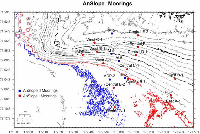
Figure cm-1

Figure cm-2

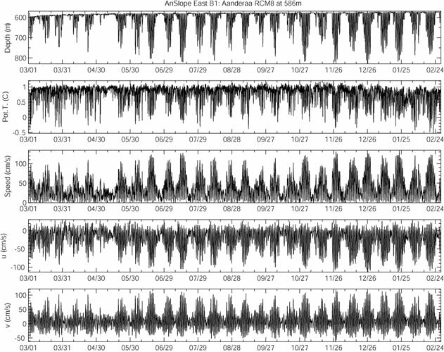
TABLE cm-1

---------------------------------------------------------------------------

MOORING LONGITUDE LATITUDE BOTTOM LONGITUDE EAST LATITUDE SOUTH

NAME (m) deg min deg min

---------------------------------------------------------------------------

ADP-1 172.5947 -71.9815 890 172 35.683 71 58.887

WEST-A 172.8263 -72.0100 609 172 49.576 72 0.604

WEST-B 172.7570 -71.9700 1025 172 45.421 71 58.199

WEST-C 172.7273 -71.9388 1630 172 43.642 71 56.326

CENTRAL-A 172.9540 -72.1617 505 172 57.236 72 9.699

CENTRAL-B1 173.1027 -72.0640 549 173 6.164 72 3.835

CENTRAL-B2 172.9417 -72.0947 525 172 56.500 72 5.681

CENTRAL-C 173.0928 -72.0307 651 173 5.568 72 1.840

CENTRAL-D 173.1908 -71.9815 1118 173 11.446 71 58.887

CENTRAL-E1 173.2125 -71.9542 1407 173 12.750 71 57.250

CENTRAL-E2 173.2115 -71.9138 1772 173 12.689 71 54.830

EAST-B 173.6282 -72.0640 982 173 37.689 72 3.843

PG-1 173.5783 -72.1203 627 173 34.696 72 7.223

EAST-A 173.5860 -72.1285 597 173 35.157 72 7.708

M1 172.6953 -72.0968 498 172 41.724 72 5.806

ADP-2 172.8995 -72.0663 537 172 53.967 72 3.983

M2 173.0665 -72.0610 541 173 3.993 72 3.657

M3 173.0007 -72.0025 664 173 0.040 72 0.146

M4 172.9170 -71.9778 1002 172 55.019 71 58.674

M5 172.9222 -71.9072 1756 172 55.331 71 54.434

---------------------------------------------------------------------------

MOORING DEPLOYMENT RECOVERY

NAME DATE DATE

---------------------------------------------------------------------------

ADP-1 6 March 2003 27 February 2004

WEST-A 6 March 2003 26 February 2004

WEST-B 6 March 2003 27 February 2004

WEST-C 4 March 2003 27 February 2004

CENTRAL-A 2 March 2003 26 February 2004

CENTRAL-B1 3 March 2003 23 March 2003

CENTRAL-B2 25 March 2003 26 February 2004

CENTRAL-C 3 March 2003 27 February 2004

CENTRAL-D 2 March 2003 27 February 2004

CENTRAL-E1 3 March 2003 22 March 2003

CENTRAL-E2 24 March 2003 28 February 2004

EAST-B 1 March 2003 28 February 2004

PG-1 2 March 2003 28 February 2004

EAST-A 1 March 2003 NOT RECOVERED

M1 8 March 2004

ADP-2 8-9 March 2004

M2 7 March 2004

M3 6 March 2004

M4 10 March 2004

M5 9 March 2004

---------------------------------------------------------------------------

S/N MOORING INST DEPTH SENSORS NOTES

---------------------------------------------------------------------------

2504 ADP-1 MicroCat 731 CTP 3.0k

2505 ADP-1 MicroCat 809 CTP 3.0k

1264 ADP-1 MicroCat 872 CTP 1.5k

C63 ADP-1 Sonteck 878 UVTP 1.5k

---------------------------------------------------------------------------

1542 WEST-A RCM 419 UVTP 1.0k

3123 WEST-A RCM 520 ---- 3.0k FLOODED AT DEPLOYMENT

6088 WEST-A RCM 587 UVT-

2530 WEST-A MicroCat 597 CTP 3.0k

---------------------------------------------------------------------------

3190 WEST-B RCM 432 UVTP 1.0k

5866 WEST-B RCM 632 UVTP 3.0k COMPASS PROBLEM

2536 WEST-B MicroCat 828 CTP 3.0k PRESSURE PROBLEM

(starts Oct. 16)

4916 WEST-B RCM 1004 UVT-

0419 WEST-B MicroCat 1014 CT-

---------------------------------------------------------------------------

6731 WEST-C RCM 436 --TP 1.0k* LOST ROTOR AT DEPLOY.

*OVER RANGED

5868 WEST-C RCM 629 --TP 3.0k LOST ROTOR AT DEPLOY.

2527 WEST-C MicroCat 923 CTP 3.0k PRESSURE PROBLEM

(starts Sept. 2)

2281 WEST-C RCM 1238 UVTP 5.0k

2528 WEST-C MicroCat 1428 CTP 3.0k PRESSURE PROBLEM

(starts Oct. 29)

4917 WEST-C RCM 1609 UVT-

0420 WEST-C MicroCat 1619 CT-

---------------------------------------------------------------------------

2529 CENTRAL-A MicroCat 273 CTP 3.0k

6732 CENTRAL-A RCM 377 UVTP 1.0k

5857 CENTRAL-A RCM 484 UVT-

0418 CENTRAL-A MicroCat 494 CT-

---------------------------------------------------------------------------

2537 CENTRAL-B1 MicroCat 290 CTP 3.0k

7165 CENTRAL-B1 RCM 398 --TP 1.0k LOST ROTOR AT DEPLOY.

6730 CENTRAL-B1 RCM 526 UVTP 1.0k DIRECTION PROBLEM

0719 CENTRAL-B1 SeaCat 536 CTP 2.0k

---------------------------------------------------------------------------

2535 CENTRAL-B2 MicroCat 281 CTP 3.0k

688 CENTRAL-B2 RCM 381 UV-

6730 CENTRAL-B2 RCM 502 --- LOST ROTOR AT DEPLOY.

0719 CENTRAL-B2 SeaCat 512 CTP 2.0k

---------------------------------------------------------------------------

2531 CENTRAL-C MicroCat 349 CTP 3.0k

6733 CENTRAL-C RCM 449 UVTP 3.0k

7214 CENTRAL-C RCM 551 UVTP 1.0k

5859 CENTRAL-C RCM 630 UVT-

0421 CENTRAL-C MicroCat 639 CT-

---------------------------------------------------------------------------

2532 CENTRAL-D MicroCat 403 CTP 3.0k

6737 CENTRAL-D RCM 508 UVTP 1.0k* OVER RANGED

1534 CENTRAL-D RCM 716 UVTP 5.0k U,V GAP

(Oct 12-Nov 13)

2533 CENTRAL-D MicroCat 910 CTP 3.0k PRESSURE PROBLEM

(starts May 9)

5860 CENTRAL-D RCM 1097 --T- LOST ROTOR AT DEPLOY.

0422 CENTRAL-D MicroCat 1107 CT-

---------------------------------------------------------------------------

2534 CENTRAL-E1 MicroCat 96 CTP 3.0k

7162 CENTRAL-E1 RCM 198 UVTP 1.0k

1540 CENTRAL-E1 RCM 412 UVTP 5.0k

2535 CENTRAL-E1 MicroCat 700 CTP 3.0k

5862 CENTRAL-E1 RCM 1030 UVTP 5.0k

2526 CENTRAL-E1 MicroCat 1205 CTP 3.0k

5861 CENTRAL-E1 RCM 1386 UVT-

0423 CENTRAL-E1 MicroCat 1396 CT-

---------------------------------------------------------------------------

2534 CENTRAL-E2 MicroCat 354 CTP 3.0k

7162 CENTRAL-E2 RCM 461 UVTP 1.0k* OVER RANGED

1540 CENTRAL-E2 RCM 677 UVTP 5.0k U,V DATA GAPS

(starting Dec 18)

2537 CENTRAL-E2 MicroCat 965 CTP 3.0k

6087 CENTRAL-E2 RCM 1266 --T- LOST ROTOR AT DEPLOY.

2526 CENTRAL-E2 MicroCat 1468 CTP 3.0k

5861 CENTRAL-E2 RCM 1751 UVT-

0423 CENTRAL-E2 MicroCat 1761 CT-

---------------------------------------------------------------------------

7769 EAST-B RCM 367 --TP 1.0k* LOST ROTOR AT DEPLOY.

* OVER RANGED

2268 EAST-B RCM 586 UVTP 5.0k

5900 EAST-B RCM 961 UVT-

0425 EAST-B MicroCat 971 CT-

---------------------------------------------------------------------------

0711 BPR SeaCat 626 CTP PRESSURE PROBLEM

(starts Jan. 21, 2004)

---------------------------------------------------------------------------

2528 M1 MicroCat 247 CT-

6732 M1 RCM 248 UVTP 1.0k

2537 M1 MicroCat 397 CTP 3.0k

751 M1 RCM 398 UVT-

5900 M1 RCM 478 UVT-

0425 M1 MicroCat 488 CT-

---------------------------------------------------------------------------

C180 ADP-2 Sonteck 521 UVTP 1.5k

1264 ADP-2 MicroCat 522 CTP 1.5k

0419 ADP-2 MicroCat 527 CT-

---------------------------------------------------------------------------

0719 M2 SeaCat 290 CTP 2.0k

5859 M2 RCM 291 UVT-

2535 M2 MicroCat 440 CTP 3.0k

1536 M2 RCM 441 UVT-

4916 M2 RCM 521 UVT-

0423 M2 MicroCat 531 CT-

---------------------------------------------------------------------------

2504 M3 MicroCat 363 CTP 3.0k

10114 M3 RCM 364 UVT-

2532 M3 MicroCat 463 CTP 3.0k

9806 M3 RCM 464 UVT-

2527 M3 MicroCat 564 CT-

7408 M3 RCM 644 UVT-

0420 M3 MicroCat 654 CT-

---------------------------------------------------------------------------

2534 M4 MicroCat 398 CTP 3.0k

5868 M4 RCM 399 UVTP 3.0k

2505 M4 MicroCat 598 CTP 3.0k

7165 M4 RCM 599 UVT-

2531 M4 MicroCat 798 CTP 3.0k

5873 M4 RCM 799 UVT-

5865 M4 RCM 979 UVT-

0421 M4 MicroCat 989 CT-

---------------------------------------------------------------------------

2526 M5 MicroCat 455 CTP 3.0k

7214 M5 RCM 456 UVTP 3.0k

2530 M5 MicroCat 655 CTP 3.0k

5856 M5 RCM 656 UVT-

2536 M5 MicroCat 1055 CT-

2281 M5 RCM 1056 UVTP 5.0k

2529 M5 MicroCat 1555 CTP 3.0k

1531 M5 RCM 1556 UVT-

1236 M5 RCM 1736 UVT-

0418 M5 MicroCat 1746 CT-

---------------------------------------------------------------------------

Final correction, reduction and management of all data collected on AnSlope moorings will be performed at the Buoy Group of Oregon State University (httpd:// kepler.coas.oregonstate.edu).

2.3 XBT/XCTD Section

Toward the end of the cruise we got a request from N. Wienders and K. Speer at FSU for salinity data in the vicinity of recent ARGO float surfacing positions for calibration purposes. Since there was not enough time to stop for CTD stations but 7 spare XCTDs were available and since we were planning on a XBT section across the ACC it was decided to combine the two. 84 T-7 XBTs (760m maximum depth), 1 XCTD (1000m) and 6 XCTD deep (1850m) were used. Figure [XBT-1] shows the drop positions (circles for XBTs, crosses for XCTDS) as well as the locations of recent ARGO-float fixes (red/yellow bullets). XBT/XCTD drops were carried out every 10 minutes of latitude between 67S and the edge of the New Zealand EEZ at 55:10S. XCTDs were substituted for XBTs near float-surfacing positions.

Out of the 7 available XCTDs only a single one was recognized by the launch computer. It was launched at 58:30S and failed at 525m, above its pressure-point calibration trigger. (According to the online manual, XCTDs use a calibrated pressure trigger that sends a signal at a predetermined depth. If that signal is received by the logging computer the depth, usually calculated from the drop speed, can be improved. For float-calibration purposes the depth correction is not important because the calibrations can be carried out in T/S or, preferably, in T/conductivity space. Uncalibrated depths are expected to be as accurate as those from XBTs. In none of the XCTDs used the pressure-point calibration worked.) When the remaining, apparently broken, XCTDs were tested using a launcher directly connected to the logging computer (bypassing the wiring inside the ship) all of them were recognized without problems. Therefore, the logging computer was moved to the wet lab and the remaining 6 XCTDs were deployed near the latitudes of the last known float positions. Launch sucess rate was 100%, although 3 XCTDs failed during descent (at 525m, 1409m, and 416m).

Based on T/S comparisons of nearby station pairs the XCTD salinities are consistent to within 0.05 or better. The T/S data of XCTD station 230 and WOCE P14 station 10 (done in 1997, 50km away) are consistent to within approximately 0.01--0.02 in salinity.

The figure below is derived from the unprocessed T-7 XBT probes launched during the section, color coded for temperature. Each profile is offset by 1°C. Profile spacing is nominally 10 nmile.

2.4 TIDE-sADCP

(G. Budillon)

The data collected by the ship ADCP have been processed in order to filter the tide component.

The applied method assumes that the characteristic of tide doesn't changes significantly in a limited area and consequently the data collected in such area can be used as a single time series as if they had been measured in a single point (like with a fixed currentmeter). The analysis of the tide has been performed using the software “T_Tide” (Pawlowicz et al., 2002).

Such procedure has been applied for all the data collected by the sADCP during the cruise selecting different geographical areas, but only for those acquired in the mooring area and off Cape Adare we obtained satisfactory results. Actually only in this limited area we collected enough data, for more than two weeks during the CTD and mooring operations, to separate the tide cycles from the measured sADCP current.

The most significant results have been obtained in the subsurface layers and averaging all the sADCP data available (layer 031-425 m).

Figure XX shows the measured (red) and residual (measured-tide; black) currents in the mooring area for the whole measured water column revealing along the slope the presence of a strong north-westward flows which follow the isobath. Over and outside the shelf the currents are less strong.

A spectral analysis of the sADCP detided current (not shown here) revealed that a not negligible energy is still present at the diurnal frequencies, for both u and v components, which most likely means that the assumption of a non-changing tide on the whole area may be not exact. Actually the worse results have been obtained in the north-west sector: the residual vectors often crossed each other, which is obviously not true.

A more careful analysis may obtain better results.

Pawlowicz R., Beardsley B., Lentz S. 2002 Classical tidal harmonic analysis including error estimates in MATLAB using T TIDE” Computers & Geosciences 28: 929–937

Figure XX – Ship ADCP velocities averaged in the layer 031-425 m (top, red vectors) and residual velocities (bottom, black vectors).

Using the velocities measured by the sADCP we have discriminated the casts performed during northward and southward flows in the Mooring Area. Analyzing the bottom temperature (deeper 5 dbar averaged) we observed (Figure YY) a significant modification during these two conditions. Actually during the southward flow the -1.0 isotherm is confined in the inner part of the shelf while with a northward flow it moves northward. In addition two apparent tongues of cold water happen during the northern flows in correspondence of stations 83 and 31.

Figure YY – Comparison between the bottom temperature measured during northward (blue) and southward (red) flows.

2.5 MOORING G - CLIMA

(G. Budillon)

The Italian mooring “G” has been deployed on February 6th 2003 at 72° 24.057’S and 173° 05.066’E at a depth of 512 m - in the Drygalski trough south of the AnSlope mooring array – several miles northward respected to the planned deployment location cause the presence of the iceberg C-19 and ice conditions. This mooring, composed by two Aanderaa RCM9 (426 and 495 m) and a temperature and conductivity recorder SBE 37 (502 m) has been recover and re-deployed on January 2004 by the Italian group and some analyses of the data has been performed during the AnSlope II cruise.

The current meter at 426 m measured an averaged northward speed of 0.12 ms^-1 on the whole period characterized by a high variability (std = 0.38 ms^-1) mostly due to the diurnal tide.

The analysis of the tide revealed that the most energetic components are K1 and O1; using the five most important constituents (O1, K1, P1, Q1, and M2 respectively) one can predict more than 90% of the original variance.

Comparing the current and thermohaline data collected at 426 m we detected repeated “warm episodes” over all the measured period as show by the Theta/S diagram (Figure ZZ) which are possibly related with the north-south shift of the slope front or with warm tongues of modified CDW (MCDW) which “pierces” the thermal front intruding over the shelf. Such intrusions have been already detected in previous surveys but nothing was known on their recurrence and persistence.

Figure ZZ – Theta/S diagram at 426 m, Mooring G (February 2003 – January 2004).

As shown in Figure WW such “warm episodes” are generally related, as expected, with the diurnal tide. During the neap tide periods they may be persistent (red arrows) or they can completely disappear (blue arrows). Such behaviour is obviously associated to the energetic contribution of longer periods which modulate the dynamic of the slope front.

Figure WW – Time series (100 days) at 426 m, Mooring G; measured (blue), tidal (green), and residual (red) components. Red and blue arrows show respectively the presence and the absence of the warm intrusions during the neap tides.

The rotary spectrum analysis of the residual (measured-tidal) current (Figure KK) suggests that the contribution of energy between 5 and 20 days (particularly at 10 days) may play an important role in modulating the behaviour of the frontal dynamics. Moreover are still present some peaks with not negligible energy - in the anti-clockwise component – with a period of about 24 hours. They can be explained with the presence of few tidal components still present in the residual current also after filtering the tide or with the presence of ≈24 hours periods of non-astronomical origin.

The contribution of components with period less than 20 hours, included the inertial currents, appears to be not significant.

Figure KK – Rotary Spectrum of the residual (measured-tidal) current: top clockwise, bottom anti-clockwise component. Aanderaa at 426 m, Mooring G (February 2003 – January 2004).

3 Appendices

3.1 Station maps

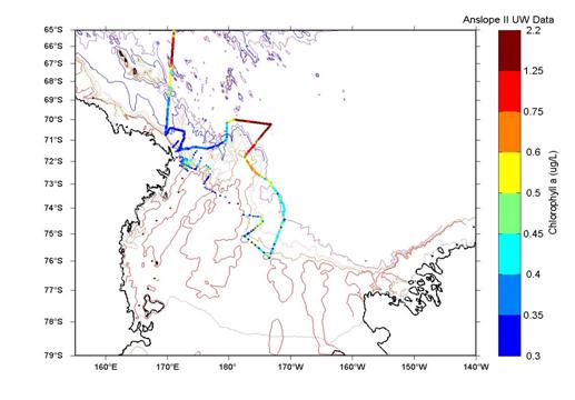
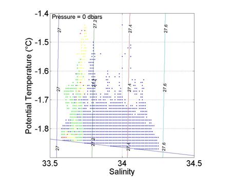
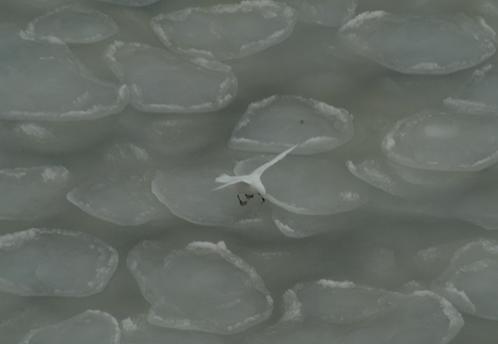
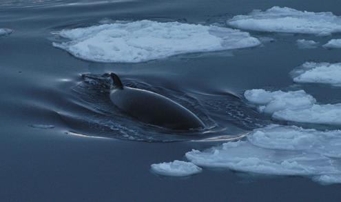
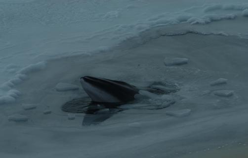
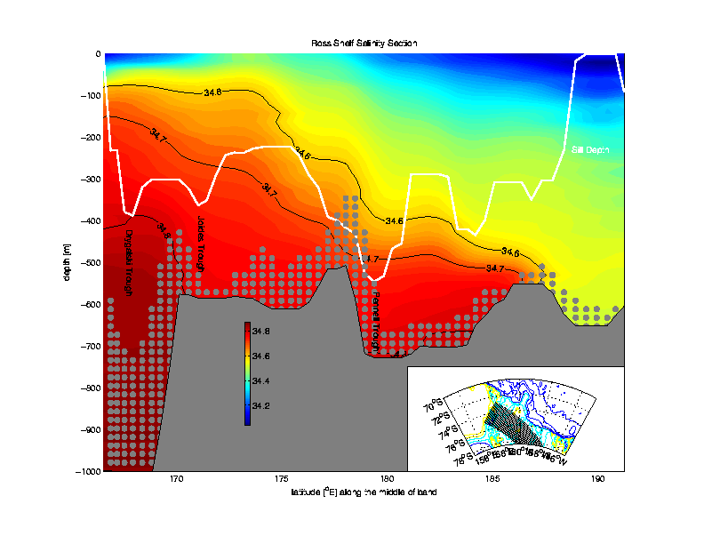
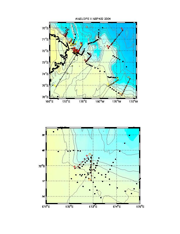
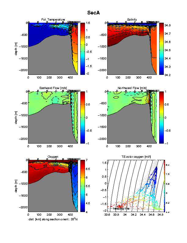
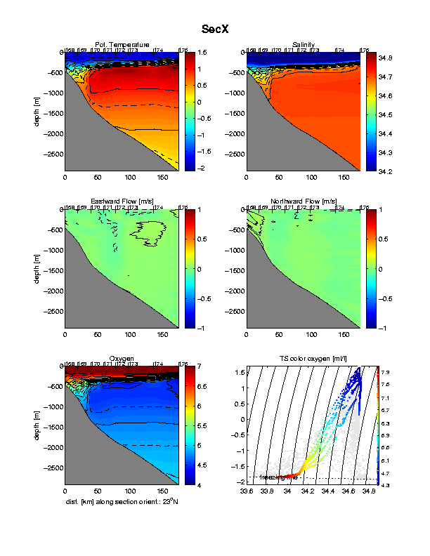
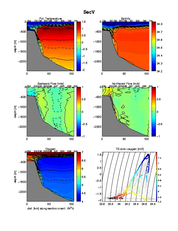
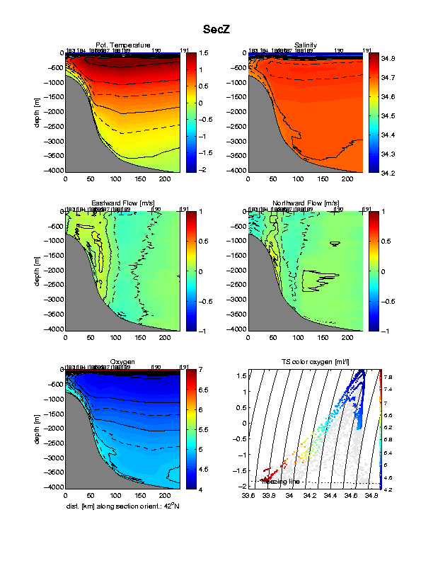
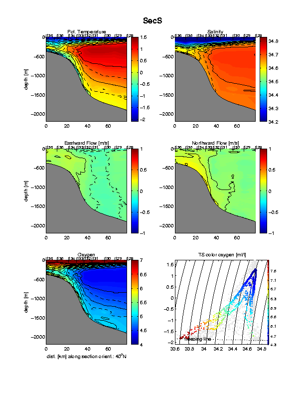
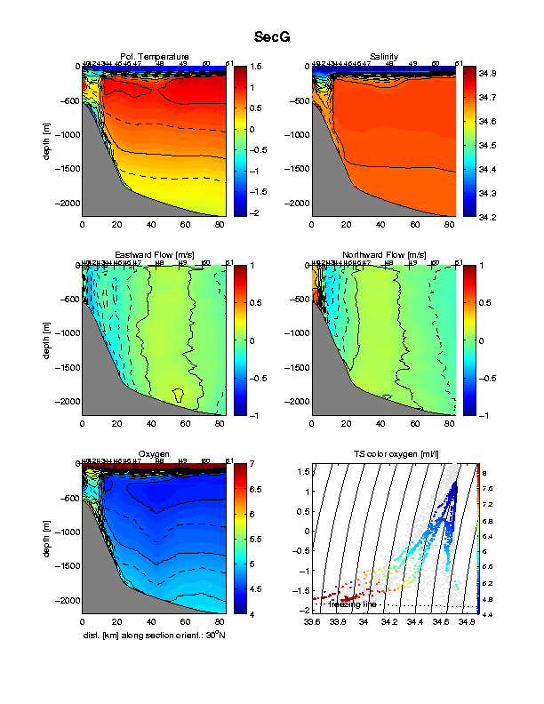
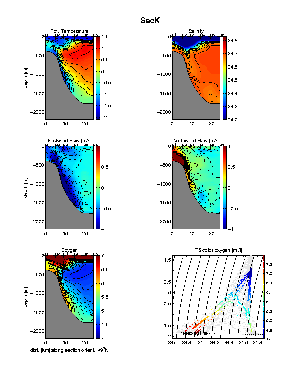
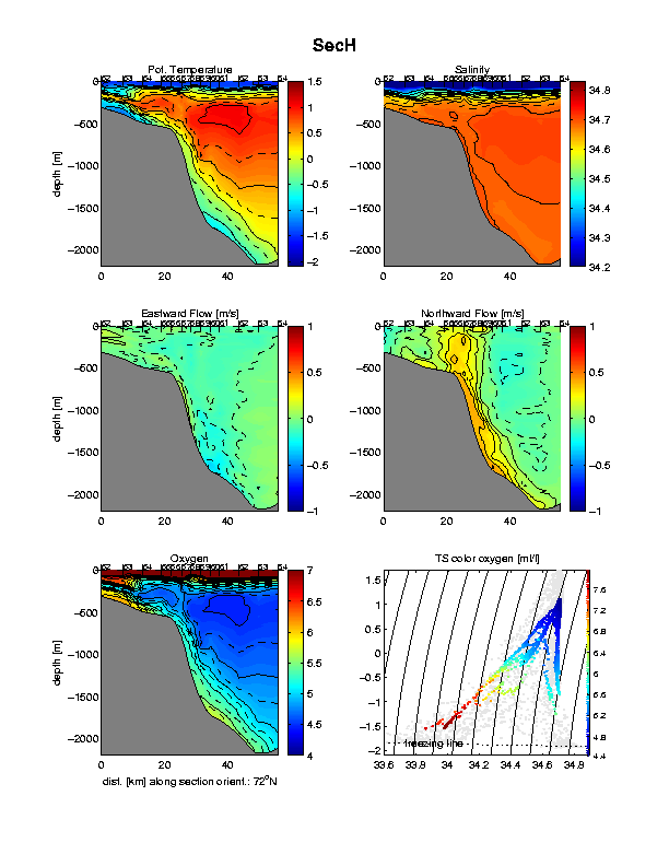
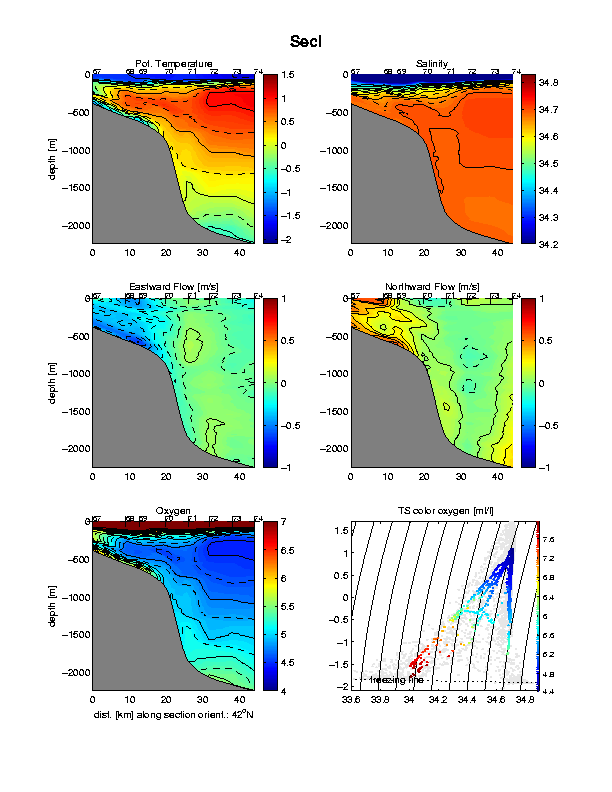3.2 Table A-1 NBP04-02 CTD/LADCP Stations

	Latitude (S)		Longitude						Water Samples						Notes
CTD	Deg	Min	Deg	Min		Date m/d/y	Time (z)	Max Pres	He	CFC	Ox	Trit	O18	Sal

1	77	29.808	165	28.476	E	02/23/04	11:39	747			8			8
2	76	36.234	167	58.716	E	02/23/04	20:59	777	4	8	8	4	4	8
3	76	00.018	167	30.276	E	02/24/04	02:43	603	13	14	14	13	13	14
4	75	00.354	166	00.006	E	02/24/04	12:49	1026		4	8			8
5	74	29.904	168	15.132	E	02/24/04	19:12	901			8			8
6	74	00.030	170	29.574	E	02/25/04	03:22	634
7	73	19.956	171	49.908	E	02/25/04	10:09	515			12			12
8	72	44.952	172	26.274	E	02/25/04	16:20	559
9	72	24.996	173	19.902	E	02/25/04	20:57	498			6			6
10	72	21.852	173	04.536	E	02/25/04	22:25	507
11	72	18.990	172	51.384	E	02/25/04	23:44	526	4	4	6	4	4	6
12	72	16.212	172	34.674	E	02/26/04	01:41	515
13	72	13.050	172	20.496	E	02/26/04	03:37	382
14	72	10.080	172	04.986	E	02/26/04	05:22	400			6			6
15	72	07.932	172	30.654	E	02/26/04	07:03	464
16	72	09.036	172	41.802	E	02/26/04	08:18	493			6			6
17	72	09.984	172	49.200	E	02/26/04	09:34	495
18	72	11.556	172	55.272	E	02/26/04	10:38	505			6			6
19	72	13.074	173	00.492	E	02/26/04	12:02	497
20	72	16.404	173	05.796	E	02/26/04	13:36	506
21	72	19.080	173	09.990	E	02/26/04	14:59	517			6			6
22	72	07.842	172	56.262	E	02/26/04	18:12	506
23	71	51.966	172	57.492	E	02/27/04	05:23	1879
24	71	54.180	172	56.004	E	02/27/04	07:42	1777	6	6	12	6	6	12
25	71	56.514	172	55.680	E	02/27/04	10:20	1485
26	71	59.244	172	55.002	E	02/27/04	12:20	891	4	5	5	4	4	5
27	72	01.092	172	55.320	E	02/27/04	13:57	599
28	72	03.216	172	57.552	E	02/27/04	15:19	531
29	72	04.950	172	54.900	E	02/27/04	16:22	516
30	72	03.054	173	02.442	E	02/27/04	17:29	535			6			6
31	72	00.012	173	07.146	E	02/27/04	19:21	954
32	71	54.000	173	14.928	E	02/28/04	03:29	1870			6			6
33	71	56.094	173	12.588	E	02/28/04	05:41	1612
34	71	57.906	173	10.506	E	02/28/04	07:46	1247
35	71	59.820	173	10.140	E	02/28/04	09:37	1004			6			6
36	72	01.650	173	06.672	E	02/28/04	11:35	705
37	72	03.906	173	04.950	E	02/28/04	13:07	536
38	72	05.754	173	13.806	E	02/28/04	14:24	537
39	72	07.170	173	21.942	E	02/28/04	15:42	547
40	72	08.898	173	31.872	E	02/28/04	16:57	545	4	8	8	4	4	8
41	72	10.512	173	41.796	E	02/28/04	18:21	550
42	72	06.906	173	32.190	E	02/28/04	22:26	624	4	8	8	4	4	8
43	72	04.854	173	38.970	E	02/29/04	06:24	878	5	12	6	5	5	6
44	72	02.898	173	43.356	E	02/29/04	08:16	1149	7	15		7	7
45	72	00.012	173	47.166	E	02/29/04	10:29	1470	7	15	16	7	7	16
46	71	57.438	173	51.102	E	02/29/04	12:56	1770	7	15	6	7	7	6
47	71	54.960	173	57.126	E	02/29/04	15:33	1871	2	2	2	2	2
48	71	48.648	174	07.974	E	02/29/04	18:40	2002	5	10	5	5	5	5
49	71	42.408	174	20.340	E	02/29/04	21:39	2119	2	2	3	2	2		rough conditions - data spiking
50	71	36.264	174	32.310	E	03/01/04	00:41	2203	5	10	6	5	5	6	rough conditions - data spiking
51	71	29.976	174	44.976	E	03/01/04	03:50	2249	2	2	3	2	2	3	rough conditions - data spiking. Wire damaged near end termination.
52	71	33.462	171	19.650	E	03/01/04	17:46	317	4	6	6	4	4	6	reterminate prior to cast
53	71	31.818	171	30.174	E	03/01/04	19:09	395
54	71	30.924	171	40.470	E	03/01/04	20:18	502	4	6	6	4	4	6
55	71	30.006	171	50.208	E	03/01/04	21:44	549
56	71	29.454	171	54.912	E	03/01/04	22:45	577	6	12		6	6
57	71	28.830	172	00.402	E	03/02/04	00:13	810
58	71	28.494	172	04.962	E	03/02/04	01:56	1210	7	12		7	7
59	71	27.930	172	10.080	E	03/02/04	04:24	1558	9	11		9	9
60	71	27.534	172	15.378	E	03/02/04	06:59	1750	9	11	6	9	9	6
61	71	27.012	172	20.010	E	03/02/04	09:40	1812
62	71	26.052	172	30.078	E	03/02/04	11:46	1990	9	18	6	9	9	6
63	71	25.002	172	39.882	E	03/02/04	14:33	2214
64	71	24.024	172	49.854	E	03/02/04	16:53	2148	9	18	7	9	9	6
65	71	27.822	172	18.000	E	03/02/04	22:32	1745
66	71	20.214	170	59.466	E	03/03/04	05:44	406
67	71	19.968	170	55.152	E	03/05/04	07:53	392
68	71	16.404	171	05.286	E	03/05/04	09:20	570			6			6
69	71	15.588	171	11.556	E	03/05/04	10:58	636
70	71	12.516	171	18.726	E	03/05/04	12:35	875			6			6
71	71	09.894	171	25.632	E	03/05/04	14:20	1892
72	71	07.512	171	31.926	E	03/05/04	16:26	2105
73	71	04.944	171	38.742	E	03/05/04	18:42	2205			6			6
74	71	02.460	171	44.862	E	03/05/04	21:21	2294		12	6			6
75	71	48.864	171	31.962	E	03/06/04	05:51	312
76	71	48.660	171	56.346	E	03/06/04	07:47	625
77	71	48.594	172	02.526	E	03/06/04	09:07	707			6			6
78	71	48.054	172	10.356	E	03/06/04	12:26	791			6			6
79	71	48.366	172	22.026	E	03/06/04	15:12	1642
80	71	48.594	172	27.636	E	03/06/04	17:14	1601
81	72	02.094	172	14.058	E	03/07/04	06:53	399
82	72	00.918	172	22.794	E	03/07/04	08:20	509			6			6
83	71	59.040	172	26.400	E	03/07/04	09:52	1147
84	71	56.940	172	33.210	E	03/07/04	12:06	1601			6			6
85	71	54.756	172	38.436	E	03/07/04	14:34	1805
86	71	54.132	172	47.496	E	03/07/04	17:26	1811			6			5
87	71	53.424	172	54.858	E	03/07/04	21:48	1839
88	71	56.100	172	53.898	E	03/08/04	00:11	1695
89	71	57.150	172	54.018	E	03/08/04	02:31	1539			6			6
90	71	59.334	172	54.318	E	03/08/04	04:56	942
91	72	01.560	172	53.418	E	03/08/04	06:57	569
92	72	03.498	172	52.950	E	03/08/04	08:58	524			6			6
93	72	05.604	172	53.550	E	03/08/04	10:54	501
94	72	06.894	172	47.622	E	03/08/04	12:25	491
95	72	06.870	172	38.970	E	03/08/04	13:39	489			6			6
96	72	07.050	172	32.910	E	03/08/04	14:56	489
97	72	06.984	172	27.168	E	03/08/04	16:03	429
98	72	07.170	172	16.668	E	03/08/04	17:17	361			6			6
99	72	01.800	172	27.030	E	03/09/04	09:34	93
100	72	01.530	172	25.476	E	03/09/04	10:01	471
101	72	00.528	172	32.472	E	03/09/04	11:18	589
102	71	59.118	172	35.832	E	03/09/04	12:46	927			6			6
103	71	57.582	172	40.218	E	03/09/04	14:35	1411
104	71	56.250	172	44.718	E	03/09/04	16:44	1667
105	71	54.978	172	48.816	E	03/09/04	19:02	1780			6			6
106	71	58.338	173	01.806	E	03/09/04	22:00	1089
107	71	53.760	172	54.708	E	03/10/04	01:52	1823
108	72	00.822	172	54.426	E	03/10/04	07:36	638
109	72	02.928	172	51.660	E	03/10/04	09:43	526
110	72	05.784	172	47.142	E	03/10/04	11:19	486			6			6
111	72	09.348	173	04.380	E	03/10/04	17:56	508
112	72	12.204	173	24.384	E	03/10/04	19:55	553			6			6
113	72	14.838	173	42.234	E	03/10/04	21:59	548
114	72	17.322	174	01.578	E	03/11/04	00:18	547
115	72	19.896	174	21.690	E	03/11/04	02:31	512
116	72	21.792	174	37.716	E	03/11/04	04:18	486			6			6
117	72	18.048	174	44.196	E	03/11/04	05:49	523
118	72	14.004	174	50.754	E	03/11/04	07:20	903
119	72	10.770	174	58.134	E	03/11/04	09:17	1175
120	72	07.182	175	05.934	E	03/11/04	11:29	1408			6			6
121	72	03.414	175	13.248	E	03/11/04	13:50	1626
122	71	59.766	175	19.116	E	03/11/04	16:03	1790			18			12
123	71	50.994	175	25.188	E	03/11/04	18:51	2037
124	72	10.956	176	23.952	E	03/12/04	00:17	1316
125	72	14.856	176	38.832	E	03/12/04	02:55	1269			6			6
126	72	17.784	176	49.152	E	03/12/04	05:07	1807
127	72	20.418	177	01.122	E	03/12/04	07:47	1992							no return to sfc after soak due to ice
128	72	26.808	177	23.790	E	03/12/04	11:40	1934		12	6			6
129	72	31.440	177	10.788	E	03/12/04	14:55	1832
130	72	35.694	176	58.674	E	03/12/04	17:40	1745		11	6			6
131	72	40.662	176	44.622	E	03/12/04	21:07	1585		10	6			6	bottle log sheet missing
132	72	43.830	176	35.928	E	03/12/04	23:46	1350		10
133	72	46.920	176	27.852	E	03/13/04	02:14	913		8	6			6
134	72	50.094	176	18.252	E	03/13/04	04:43	602		6
135	72	54.684	176	05.262	E	03/13/04	06:30	453
136	72	59.148	175	53.832	E	03/13/04	08:46	384		6	6			6
137	73	07.812	176	05.622	E	03/13/04	12:04	362
138	73	11.082	176	29.634	E	03/13/04	14:06	408
139	73	14.628	176	54.336	E	03/13/04	16:39	454
140	73	18.054	177	18.840	E	03/13/04	18:28	479			6			6
141	73	21.588	177	43.980	E	03/13/04	20:54	458
142	73	29.532	178	34.434	E	03/14/04	01:14	371
143	73	32.748	179	27.108	E	03/14/04	05:18	363		6	6			6
144	73	46.830	179	56.124	W	03/15/04	00:26	339		6
145	73	49.620	178	35.406	W	03/15/04	16:05	440		7	6			6	new pump on primary sensors. Discovered that orig pump was low flow model.
146	74	20.184	177	14.898	W	03/16/04	10:36	632	3	6		3	3
147	74	15.930	177	34.464	W	03/16/04	21:15	575		5				5
148	74	19.398	176	51.924	W	03/17/04	04:20	762		6	6			6
149	74	17.832	176	35.850	W	03/18/04	06:40	851	4	8		4	4
150	74	20.082	176	03.414	W	03/18/04	09:57	1411	6	12		6	6
151	74	20.790	175	41.814	W	03/18/04	13:14	1912	7	14	12	7	7	12
152	74	20.658	175	19.338	W	03/18/04	16:23	2306	7	14		7	7
153	74	21.204	174	46.890	W	03/19/04	03:02	2671	7	14	6	7	7	6
154	74	32.616	174	32.352	W	03/19/04	11:44	2537		2
155	74	37.086	174	56.352	W	03/19/04	16:48	2428		12	12			12
156	74	42.396	175	23.016	W	03/19/04	21:04	2267		2
157	74	47.106	175	45.678	W	03/20/04	03:14	2113		12	6			6
158	74	51.756	176	08.394	W	03/20/04	06:57	1886		12
159	74	54.762	176	25.980	W	03/20/04	10:10	1756		10
160	74	58.068	176	47.526	W	03/20/04	13:44	1119	2	10	10	2	2	6
161	75	01.026	177	02.862	W	03/20/04	16:08	482		7
162	75	05.718	177	30.816	W	03/20/04	18:25	446		8
163	75	12.456	176	52.704	W	03/20/04	21:01	538		8	6			6
164	75	19.290	176	18.396	W	03/20/04	23:34	556	1	6
165	75	25.704	175	45.948	W	03/21/04	02:09	564		6
166	75	32.526	175	10.548	W	03/21/04	05:18	527		6	6			6
167	75	41.928	174	22.662	W	03/21/04	08:40	485		6
168	75	53.088	173	27.174	W	03/21/04	12:17	477		6
169	75	43.686	173	12.918	W	03/21/04	14:49	795	2	6		2	2
170	75	33.546	172	53.334	W	03/21/04	18:00	1358	6	10	5	6	6	6
171	75	23.796	172	38.658	W	03/21/04	21:18	1649		12
172	75	14.274	172	21.894	W	03/22/04	01:05	1894	6	12	6	6	6	6
173	75	04.620	172	06.360	W	03/22/04	04:42	2070		12
174	74	45.366	171	32.094	W	03/22/04	10:29	2500	6	12	6	6	6	6
175	74	26.352	171	00.672	W	03/22/04	16:10	2978		12	12			12
176	73	24.732	172	02.994	W	03/23/04	06:54	3638			6			6
177	72	56.316	173	07.536	W	03/23/04	15:29	3269		2	6			6
178	72	46.296	174	06.036	W	03/23/04	21:26	3213		12
179	72	41.328	174	35.130	W	03/24/04	06:29	2445		2
180	72	36.294	175	04.218	W	03/24/04	09:56	1525		12	6			6
181	72	31.986	175	32.730	W	03/24/04	13:02	1097		8
182	72	26.220	176	01.056	W	03/24/04	15:58	816		10	6			6
183	71	47.508	177	26.058	W	03/25/04	00:37	785		2
184	71	37.350	177	06.036	W	03/25/04	03:36	987		2
185	71	28.806	176	36.690	W	03/25/04	06:32	1602	4	6	6	4	4	6
186	71	23.616	176	23.880	W	03/25/04	09:15	2402	4	8		2	2
187	71	19.080	176	09.378	W	03/25/04	12:29	2974	4	8		1	1
188	71	09.990	175	44.718	W	03/25/04	16:46	3421	4	8	6	1	2	6
189	71	01.686	175	24.882	W	03/25/04	21:17	3723		2
190	70	37.116	174	16.074	W	03/26/04	04:52	4026		2					some spikes in data below 3000 m
191	70	14.298	173	12.678	W	03/26/04	11:14	4170	5	10	12	2	4	12	many spikes in data below 3000 m, appears to depend on lowering rate
192	69	59.310	179	11.106	W	03/27/04	02:50	3696		2					new slip rings installed. spiking continues
193	70	10.176	179	41.148	E	03/27/04	08:25	3647		2	6			6	spiking continues
194	70	26.052	179	40.002	E	03/27/04	12:57	3455		2					varied lowering rate to test noise dependency on speed
195	70	34.236	179	36.978	E	03/27/04	16:51	3028		2	6			6
196	70	42.918	179	38.958	E	03/27/04	20:28	2278		2
197	70	51.216	179	37.830	E	03/27/04	23:42	1630			6			6
198	71	01.446	179	25.746	E	03/28/04	02:45	1585
199	71	04.854	179	08.976	E	03/28/04	05:20	1957
200	71	07.566	178	52.458	E	03/28/04	07:52	2499
201	71	10.662	178	37.452	E	03/28/04	10:51	2769
202	71	14.148	178	22.284	E	03/28/04	13:57	2786
203	71	15.792	178	03.390	E	03/28/04	17:20	2973			12			12
204	71	17.874	177	36.990	E	03/28/04	21:26	2705
205	71	19.560	177	19.008	E	03/29/04	00:26	2370
206	71	21.144	177	03.630	E	03/29/04	03:10	2016
207	71	22.470	176	48.294	E	03/29/04	05:41	1136
208	71	23.088	176	40.968	E	03/29/04	07:31	1829
209	71	24.408	176	32.502	E	03/29/04	09:48	2190			6			6
210	71	19.794	174	39.120	E	03/29/04	17:30	2260			6			6
211	71	26.070	172	30.360	E	03/30/04	04:09	1991			6			6
212	71	26.478	172	23.724	E	03/30/04	06:35	1888			6			6
213	71	24.714	172	13.230	E	03/30/04	09:36	1804
214	71	27.984	172	09.414	E	03/30/04	12:37	1495
215	71	28.986	172	05.082	E	03/30/04	14:31	1236
216	71	28.908	171	59.532	E	03/30/04	16:15	735
217	71	29.838	171	50.544	E	03/30/04	17:43	551
218	71	30.594	171	40.080	E	03/30/04	19:11	501			6			6
219	71	22.650	171	58.338	E	03/30/04	22:55	1526
220	71	17.592	172	13.170	E	03/31/04	02:37	2143			6			6
221	71	10.638	172	18.828	E	03/31/04	05:39	2350
222	71	03.546	172	28.830	E	03/31/04	09:05	2340
223	70	53.010	172	46.224	E	03/31/04	13:17	2396
224	70	34.956	172	44.952	E	03/31/04	17:56	2510			12			12
225	70	25.506	170	24.618	E	04/01/04	03:59	2633
226	70	31.938	170	10.740	E	04/01/04	07:31	2541			6			6
227	70	35.970	170	04.596	E	04/01/04	10:42	2479
228	70	38.796	169	57.756	E	04/01/04	14:03	1830
229	70	41.028	169	55.422	E	04/01/04	16:17	1187
230	70	44.076	169	49.260	E	04/01/04	18:20	664			6			6
231	70	46.758	169	44.082	E	04/01/04	20:05	338
232	69	59.886	169	59.832	E	04/02/04	05:12	2739

Total Samples									216	700	640	204	207	624

4 Ancillary Program Reports

4.1 AnSlope - Phytoplankton Biomass Ancillary Project

Erin Stone

Oceanic fronts, and the Antarctic shelf-slope front (ASF) region in particular, are areas of known high productivity. Indications that the ASF is a region of higher biological productivity include observations of larger populations of krill, sea birds, whales, and seals, but there are few quantitative observations of primary producers. It is the objective of this project to characterize the spatial variability of late austral summer to austral autumn season (Feb-Apr) phytoplankton biomass in the Ross Sea, ASF region within a detailed hydrographic framework. To this end, measurements included chlorophyll a concentrations, both underway and on-station, and phytoplankton enumeration via epi-fluorescent slides. The biological measurements taken during the cruise will be correlated to the physio-chemical data collected including Lowered Acoustic Doppler Profiling (LADCP) of currents, and measurements of temperature, salinity, and dissolved oxygen. These physio-chemical measurements establish the regional hydrography within which the phytoplankton biomass data may be interpreted. Further work will include the epifluorescent enumeration as well as comparison of in situ chlorophyll data to satellite ocean color data (SeaWIFs).

The phytoplankton biomass data was collected to test two main hypotheses, which attempt to explain the increased biological activity at the ASF. The first is the convergent nature of the front brings together water masses and their accompanying biota, which accumulates populations of phytoplankton and krill, which could support the higher trophic levels in the ASF region. The other is that deeper stratification of waters in the region may allow for increased water column stability enabling higher phytoplankton growth rates which would also support higher trophic levels. Both of these hypotheses may be tested using data collected during this cruise. To support or reject these hypotheses, the objectives include quantifying the distribution of phytoplankton across the Antarctic Slope Front Region; and correlating the biological variables with the physio-chemical properties of the Antarctic Slope Front including current direction and speed, and the definition of local water masses.

Methods

On-Station and Underway Sample Collection

Seawater was collected at selected stations using a rosette of 24 10L Niskin bottles from 5m to the surface. In addition to the bottles, the rosette was equipped with a Sea-Bird Electronics CTD and Oxygen Sensor, a Wetlabs C-Star Transmissometer, a Biospherical Instruments Underwater PAR sensor, a Wetlabs Fluorometer (calibrated 7 months before the cruise). All instruments were calibrated 4-5 months before the cruise unless otherwise indicated. Samples were taken from the Niskins using a 1 Liter Nalgene bottle rinsed then filled with the seawater sample. From this liter, 550ml was partitioned for fluorometric chlorophyll aanalysis, and 300 ml was separated for making slides for later Epifluorescent enumeration.

Samples were taken from the underway system just upstream from the underway fluorometer for fluorometric and epifluorescent analysis. The underway Fluorometer is a Turner Designs 10AU unit. It was discovered on day 21 of the cruise that the underway fluorometer was experiencing wide and unaccountable swings in raw voltage values. The fluorometer was investigated and condensation was found on the outside of the cuvette. The cuvette and compartment were dried and new desiccant was added to the compartment before it was resealed. The underway fluorometer voltage data from Julian Days 54 - 79 is not reliable for use due to this problem.

Pigment Analysis

Discrete Chl a measurements were made by filtering 550 ml seawater, taken from both the Niskin bottles and the underway system, onto 25-mm GF/F filter pads and extracting the pigments in 90% acetone for 24 hours. Samples were vortexed briefly before and after extraction then centrifuged before fluorescence to remove filter particles from the extract. Chlorophyll a (Chl a) + Phaeophytin a (phaeo) measurements were made, then the extract was acidified with 10% HCl (hydrochloric acid) to determine the phaeo concentration. Quantification of these pigments were made using a Turner Designs 10AU bench-top unit. The fluorometer was calibrated at the beginning, middle and end of the cruise using an on-board spectrophotometer to measure the concentration of a purified Chlorophyll-a standard purchased commercially (Sigma). The discrete fluorometric results from station and underway samples were used to calibrate both the underway voltages and the data from the CTD mounted fluorometer. The calibration curve relating Chl a (ug/L) to underway voltage (v) was Chl a (ug /L) == 0.5252*(UW voltage), r² = 0.9065, n=137. The curve relating CTD fluorometer pigment concentrations to discrete concentrations is Chl a (ug /L) = 0.2373*(CTD Chl a (ug /L)) + 0.2701, r² = 0.827, n=23.

Epifluorescent Slide Making

The 300 ml of sample water partitioned for slide making was further divided into a 50ml and 250 ml sample. The 50 ml sample was fixed with 2ml paraformaldehyde and stained with 40 μl proflavine. The 250 ml sample was fixed with 250 μl alkaline lugols, 2ml Borate-Buffered Formalin, 750 μl sodium thiosulfate and then fixed with 200 μl proflavine. These fixed samples set for 1 hour in a 5^o C. cooler. The 50 ml samples were condensed via filtration onto 0.1 μm black polycarbonate filters. The 250 ml samples were filtered onto black polycarbonate 0.5 μm filters. With approximately 5 ml of fixed seawater left, 1 ml 4,6-diamidino-2-phenyl indole (DAPI) was added to the remaining seawater to stain the planktonic cells on the filters. These filters were mounted on glass slides with Type FF immersion oil, covered with a cover slip and allowed to sit in the dark for 10 minutes. Once set, the slides were kept frozen at –70^o C for preservation to later analyze and enumerate using epi-fluorescent microscopy at Lamont-Doherty Earth Observatory.

Whole Water Samples

Whole water samples of 250 ml were taken at the end-members of transects conducted on the cruise. At each collection, 250 ml were treated with 1.25 ml alkaline lugols and another 250 ml was treated with 1.25 ml Borate-buffered formalin. These samples were kept chilled at 5^o C for later species identification at Lamont-Doherty.

Initial Results

The beginning of the cruise saw elevated chlorophyll alevels heading north out the Ross Sea to the ASF. These concentration values were in the range of 1-2 ug/L Chl a. Once at the shelf-slope front, Chl a values dropped to approximately 0.2-0.5 ug/L (both underway and on station data). These values were fairly consistent across the slope-front region both in and out of the ice until Julian day 84 when the values started to increase as the stations of Section Z lead the ship out of the thicker ice, through a band of pancake ice and into open water (fig 1). Chl a values in this region outside the ice peaked at 2 ug/L. At the end of Section Z (Stations 184-191), the surface water was fresher (salinity as low as 33.58 psu) and warmer (temperature as high as –1.44^oC).

Upon leaving the ice edge and heading the ship back into the ice, the underway voltage dropped down to values comparable to the previous values taken in the ice of 0.2-0.4 ug/L. These did not vary much until the ship left the ice again on Julian day 94 when they increased to 1.5 ug/L with the warmer fresher water found at the ice edge. Initially it appears that salinity (especially as an indicator of reduction in ice cover) is a more important factor in the potential for increased Chl a values (fig 2).

Further analysis of underway, on station, satellite data and the epifluorescent slides will enable a more definitive analysis of physical factors effecting phytoplankton biomass within this region.

Figure 1. Calibrated Underway Fluorometer Data (ug/L) (bathymetry = isobaths every 500m depth)

Figure 2. TS diagram of Calibrated Underway Data. green = Chl a>1.5 ug/L; yellow=Chl a > 1.75 ug/L; red=Chl a>2 ug/L

4.2 Sea Ice Observations

William H. Lipscomb Margaret Knuth

Los Alamos National Laboratory Clarkson University

The sea ice observation program was carried out by Margaret Knuth and William Lipscomb. Hourly observations were made from the bridge from 23 February-2 April 2004 while the ship was underway. These observations followed a protocol developed by Anthony Worby and others of the Antarctic Cooperative Research Centre (Worby et al., 1999). The AnSlope II sea ice observations will be added to the ASPeCt (Antarctic Sea ice Processes and Climate) data base, which contains ice observations from cruises throughout the Antarctic, as part of a program organized by the Scientific Committee on Antarctic Research.

The standard hourly ice observation included the ship’s position and an estimate of the total sea ice concentration, subdivided into one to three ice types. The thickest type was designated as primary, the next thickest as secondary, and the thinnest as tertiary. Each type was identified as frazil, shuga, grease, nilas, pancakes, young grey ice, young grey-white ice, first-year ice (thin, medium, or thick), multiyear ice, brash, or fast ice. For each ice type the concentration (on a scale of 0 to 10, where 10 = total coverage), ice thickness, floe size, topography, snow thickness, and snow type were estimated within 1 km of the ship, using standard codes from the ASPeCt protocol. The open water extent was also recorded. Supplemental information included the meteorological condition (using standard two-digit codes), air and water temperature, wind speed and direction, cloud fraction, and visibility. Short comments were added to aid in interpreting the data. This information was recorded on log sheets and entered in a data base.

Lipscomb took the first shift of each Greenwich day (0-11 Z) and Knuth the second shift (12-23 Z). When visibility permitted, a representative section of the ice was photographed from the bridge at the time of observation. When clouds or darkness restricted visibility to less than 1 km, the ice visible from the ship was observed for 5-10 minutes and assumed to be representative of the nearby ice. Observations were not made when the ship was stopped for mooring deployment/recovery or CTD casts. Also, observations were skipped when the ship was significantly slowed by poor weather or thick ice. Most of the missing observations are associated with moorings and CTD casts. We made 519 observations during 40 days, an average of about 13 per day.

The ASPeCt protocol is fairly self-explanatory and easy to use. In some cases, however, it was difficult to make precise observations or distinguish between two or more options. For the sake of uniformity, we adopted the following conventions:

Multiyear ice is defined as ice that has survived at least one melt season. We assumed that the summer melt season had ended before the cruise began, implying that all first-year ice had formed within the past few weeks. For this reason, first-year ice thicker than 50 cm was rare. The presence of algae in upper or interior ice layers was often used to identify multiyear ice.

Grease ice was assigned a standard thickness of 2 cm.

Ridges were assumed to be consolidated (code 7xy), because of the difficulty in distinguishing in a consistent way among new snow-covered ridges (code 6xy), consolidated ridges, and older weathered ridges (code 8xy).

It was difficult to distinguish among snow type 2 (cold new snow), type 3 (cold old snow) and type 4 (cold wind-packed snow). If uncertain, we labeled unsaturated snow as type 3.

Ice and snow thickness were estimated with reference to a buoy of 45 cm diameter hung from the lower starboard deck. When the ship was in open water and was not upturning ice, ice thickness was estimated based on snow thickness and earlier observations. The mean ice thickness may be systematically biased low because the ship often sought leads and thin ice for faster passage. Concentration observations were less precise when the ship was in a broad lead, because it was difficult to judge what fraction of distant floes was located within 1 km of the ship.

The ASPeCt sea ice observations were supplemented by three-hourly estimates of the number of icebergs within a radius of 6 nautical miles (nm). We relied heavily on the ship’s radar even in clear conditions, since it was often impossible to determine visually whether an iceberg on the horizon was within 6 nm. On days with poor visibility and at night, radar was used exclusively. When many icebergs (> 15) were present, we sometimes rounded to the nearest multiple of 5.

We wrote six short summaries of weekly sea ice and iceberg conditions. Edited versions of these summaries follow below.

Week 1 (February 23-28):

Leaving McMurdo, we passed through a ship-cut channel filled with young grey ice and bounded by fast ice about 300 cm thick. On the way north toward Cape Adare, nearly all ice types defined in the protocol were observed. Usually the ice cover was sparse, with small floes (20-100 m diameter), cake ice (< 20 m diameter), and brash surrounded by > 80% open water. Occasionally, we saw thick (> 100 cm) multiyear floes. There were many icebergs (> 20 within 6 nm) as the ship passed near the very large iceberg B15A on February 24, and again around 76^oS, 167^oW on February 27.

Week 2: (February 29-March 6):

Ice observations were curtailed by 48 hours of stormy weather March 3-5. Before the storm the ice concentration was usually low and often zero. When ice was present, we saw small floes (< 20 m) spanning a wide range of thicknesses. The ice types with greatest concentration were grease, brash, and thin first-year ice. After the storm the ice concentration increased to 5-10, with other ice characteristics similar to pre-storm. Many bergy bits were observed.

Week 3 (March 7-13):

Early in the week near the mooring sites, the ice concentration ranged from 5-10 in a region that had been largely ice-free a week earlier. Young grey-white ice (~20 cm) was mixed with thin first-year ice (30-50 cm) and thicker multiyear ice (80-100 cm). Most floes were small (< 100 m). We moved eastward beginning March 10 and observed nearly total ice coverage for the rest of the week. After March 12 there was a marked increase in average floe size to several hundred meters. Ice thicknesses remained in the 15-100 cm range, with a mean of about 40 cm. Between March 12 and March 13, the iceberg density dropped from 30 per 6 nm radius to near zero.

Week 4 (March 14-20):

After moving east of the Date Line on March 14, we encountered active ridging for the first time. The ship was caught in pressure for several hours on the evening of March 14, and then slowed by pressure ridges several times during the week. Sail heights of 1 m or more were common. Before March 17 wide leads were common, but for the rest of the week the concentration was almost always 10, with large floes of diameter > 500 m. By far the most common ice type was first-year ice 30-50 cm thick, with a thin (~5 cm) snow cover. Multiyear ice of thickness 80-150 cm, with a thick (~30 cm) snow cover, was often present, especially in areas of ridging.

Week 5 (March 21-27):

The ship began the week in large (> 500 m) unbroken floes of lightly ridged 40-50 cm first-year ice, covered by 3-10 cm of snow. The ice grew thinner with smaller floes as we moved north. Beginning March 22 there were more leads, smaller floes (50-500 m), and a mixture of thick (~1 m) multiyear ice with first-year ice, grease, and nilas. On March 26 the sea was covered with small pancakes (~1 m diameter or less), dramatically shaded brownish orange by algae. Pancakes then alternated with open water. On March 25 the ship passed through a field of several dozen icebergs near 71.7^oS, 177.2^oW. This was the highest concentration of icebergs seen during the cruise.

Week 6 (March 28-April 2):

The week began near the Date Line in open seas. As the ship moved west, ice concentrations were initially 7-10, increasing to 9-10 by the time we reached the mooring area near the coast. Both thick (~100 cm) multiyear ice and thinner (~40 cm) first-year ice were usually present, along with young grey ice, nilas, and/or grease in refreezing leads. Snow thickness was typically 20-40 cm on multiyear ice, but rarely exceeded 10 cm on other ice types. Conditions in the mooring area had changed considerably since week 3. This time there were larger floes (typically 100-500 m) and greater concentrations of multiyear ice (2-5). On April 2 the ship turned northward and spent several hours in a region of small floes and cake ice. The ice edge was abrupt; we observed a 90% concentration of pancakes just an hour before reaching open seas. The ship passed through a dense field of icebergs (~50 bergs in a 6 nm radius) on March 28.

References

Worby, A., I. Allison, and V. Dirita, 1999: A technique for making ship-based observations of Antarctic sea ice thickness and characteristics. Antarctic Cooperative Research Centre for the Antarctic and Southern Ocean Environment, Research Report No. 14, 63 pp.

4.3 MARINE MAMMAL PASSIVE ACOUSTIC MONITORING

Ana Širović

Introduction

Cetaceans spend a large part of their life under water and, as such, they can be difficult to observe and study from the surface. Baleen whales are known to produce low frequency, loud, repetitive calls that propagate well underwater. Since the calls of most baleen whales are unique and easily recognizable, it is possible to distinguish among various species using passive acoustic techniques. Acoustics can be used for a variety of purposes ranging from species identification to determining distribution and seasonality patterns. The main species of interest during this cruise were blue (Balaenoptera musculus), fin (B. physalus), humpback (Megaptera novaeangliae), and minke (B. bonaerensis) whales. Sperm whale (Physeter macrocephalus – an odontocete) calls can also be detected and identified to species. Calls produced by other odontocetes are more varied, tend to be higher frequency, and are more difficult to attribute to a specific species. It is also possible to recognize calls of several seal species: crabeater seals (Lobodon carcinophaga), Weddell seals (Leptonychotes weddellii), leopard seals (Hydrurga leptonyx) and Ross seals (Ommatophoca rossii).

The first goal of the acoustic monitoring effort was the deployment of two Acoustic Recording Packages (ARPs). Data from the ARPs can be used to determine distribution and seasonality of mysticete whales within the range of the recordings. The second goal was obtaining acoustic recordings of various species of marine mammals by making opportunistic deployments of sonobuoys from an underway ship. These recordings are helpful in analysis of ARP data, but also enable data acquisition outside of the range of the ARPs and can be used in conjunction with visual observations for classifying heard calls to the right species of marine mammals.

Methods

The Acoustic Recording Packages (ARPs) that were deployed during this cruise are bottom-mounted instruments with a hydrophone component floating 10 m above the mooring. Other components of the ARP are: a data logging and acoustic release systems, batteries, and flotation. The ARPs will record continuously at 1000 samples per second for 500 days and the data will be stored on two 18 Gb hard disks. The low frequency calls of blue and fin whales can be recorded from as far as 60 km radius, but somewhat higher frequency minke, humpback, southern right (Eubalaena australis) and possibly sperm whale calls should also be detectable, although over smaller ranges.

During AnSlope II, sonobuoys were deployed opportunistically in order to supplement the information that will be gathered from the seafloor recorders. Sonobuoys are expendable underwater listening devices. The sonobuoy has 4 main components: a float, a radio transmitter, a saltwater battery, and a hydrophone. The hydrophone is an underwater sensor that converts the pressure waves from underwater sounds into electrical voltages that get amplified and sent to the radio transmitter housed in the surface float. This radio signal is picked up by an antenna and a radio receiver on the ship, and it can be reviewed and simultaneously recorded as a WAV file and on a digital audiotape (DAT) at a sample rate of 48 kHz.

Two different types of sonobuoys were used during this cruise: omnidirectional and directional. Omnidirectional sonobuoys (AN/SSQ-57B and AN/SSQ-41B) have hydrophones with a frequency response from 10 to 20,000 Hz. For these types of sonobuoys hydrophone depth can be set to 90 or 400 ft (57B) and 90 or 1000 ft (41B). It is not possible to determine the location of the sound source using these sonobuoys. DIFAR (directional frequency analysis and recording; AN/SSQ-53D) sonobuoys have a hydrophone with directional detection capabilities and frequency response from 5 to 2,400 Hz. Hydrophone depth for 53D sonobuoys can be set to 90, 400, or 1000 ft. The direction of the sound relative to the sonobuoy is obtained from two pairs of direction sensors and a compass located inside the hydrophone. This kind of acoustic data can be correlated to visual observations of marine mammals. All of these sonobuoy types can transmit for a maximum of 8 h before scuttling and sinking.

Three antennae were used during the cruise: a 160 MHz omnidirectional Cushcraft Ringo Ranger ARX-2B, 162 – 174 MHz directional Yagi, and a 138 – 174 MHz dipole Sinclair SRL-210 A-2. The antennae were mounted on the science mast, 33 m above sea surface level. The average reception range of the Ringo Ranger during the cruise was 6 nm and it was 12 nm for the Yagi. It was difficult to determine the range of the Sinclair because it was facing forward, but it was more than 8 nm. This setup of the Sinclair was useful for signal reception during CTD stations. The Yagi was generally used when steaming away from the sonobuoy in a straight line, because of its narrow beam pattern, while Ringo Ranger was preferable when steaming through the ice (which was often difficult to do in a straight line). These ranges were variable depending on weather conditions.

We used software controlled ICOM IC-PCR1000 scanner radio receivers for reception of sonobuoy signal. Data were recorded as 30 minute WAV files using software program Ishmael. As a back-up, data were simultaneously recorded on digital audiotapes using Sony PCM-M1 digital audio recorder. Ishmael was also used for real-time review of the sounds. The following items were noted at each deployment: time, latitude, longitude, and depth at deployment, sonobuoy type, channel, time, and depth settings, speed and heading of the ship, ice conditions, and the reason for deployment. Data were generally reviewed in real time and notes of sounds heard were kept. If DIFAR sonobuoys were deployed, bearings to interesting sounds were calculated using Greenridge DIFAR demultiplexing software and they were noted with the description of the sound. Comments on reception and sonobuoy range were also noted. Also, if real-time data were not monitored a note was made so that data can be reviewed in post-process analysis. A spreadsheet with the following information is included on the AnSlopeII data CD: sonobuoy number, date, time and location of deployment, sonobuoy type, indication of species that was heard, reception range, reason for deployment (when applicable), and any additional comments.

The noise levels from the Nathaniel B. Palmer were high when breaking through ice, therefore many recordings had high noise. This low frequency noise made it more difficult to determine presence of baleen whale calls

Preliminary results

The Acoustic Recording Packages were successfully deployed at 62°45.1’ S and 171°31.3’ E, and 71°24.9’ S and 172°40.0’ E. The deployment depths were 2847 and 2198 m, respectively.

Sonobuoys were deployed when marine mammals were visually detected and randomly throughout the cruise, but attempting to provide maximum reception from a single sonobuoy. A total of 77 sonobuoys were deployed: 50 omnidirectional (32 57B and 18 41B) and 27 DIFAR. Average failure rate was 29%, but it differed between different sonobuoy types. DIFARs were least successful and 14 failed (52%). Omnidirectional sonobuoys had a lower failure rate (6% for 57B and 33% for 41B). This relatively high failure rate is probably due to the age of the sonobuoys, which are only given for research after their shelf life in the Navy has passed.

Locations of all the deployments as well as a preliminary summary of the sonobuoys on which calls were heard can be seen in the complete and close-up maps of the study area (Figures 1 and 2). Calls from several species were heard: blue whales, fin whales, humpback whales, killer whales (Orcinus orca), minkes, Weddell and crabeater seals. Several unidentified call types were heard. They can be classified into three categories: “80-40 Hz downsweeps” of approximately 2 s duration, series of pulses centered around 100 Hz, and “120-60 Hz downsweeps.” Even though the source of these calls is not currently known with certainty, they are most likely produced by a marine mammal. The most frequently heard calls were from odontocetes. They were heard on 11 sonobuoys, and while one of those was most likely a beaked whale, the others were probably killer whale calls. Baleen whale species heard most frequently was minke whale, and they are a likely source of “120-60 Hz downsweeps.” These calls were heard most often along the shelf edge, in ice covered areas. Humpback whale song was recorded on several occasions, mostly in the vicinity of the ice edge. Main components of the song were in the 300-500 Hz range and several themes could be distinguished in the song. Crabeater seals were heard once in the eastern part of the survey area, but Weddell seals calls were more common and they were heard seven times, predominately in the southwest of the survey area. Pulses were heard on four sonobuoys. It is possible they were produced by Ross seals, but this needs further confirmation. Fin whale calls were heard on one sonobuoy. It is possible, however, that “80-40 Hz downsweeps” were produced by fin whales as well. These calls were heard in the vicinity of the ice edge.

Further analysis of the recordings is needed to double check for calls that were possibly not detected during the preliminary review. Verification of the sources of the unidentified calls is also needed.

Figure 1. All sonobuoy deployment locations during AnSlope II. Sonobuoys on which marine mammal calls were heard are marked with an appropriate symbol (see legend).

Figure 2. Close-up of sonobuoy deployments and marine mammals heard in the core study area.

NBP 0402

4.4 CETACEAN AND WILDLIFE DIVERSITY CRUISE SUMMARY

Deborah Thiele and Debra Glasgow

International Whaling Commission

snow petrel with krill on pancake ice

INTRODUCTION

Since the 1999/2000 austral summer the International Whaling Commission (IWC) Scientific Committee has been facilitating the inclusion of cetacean research programs aboard the multidisciplinary research cruises of many nations operating in the Antarctic (e.g. CCAMLR 2000 and Southern Ocean GLOBEC 2001-3, UK, Australia, USA, Germany). IWC participation in these cruises is aimed at gathering cetacean data simultaneous with other physical and biological programs, to allow integration of cetacean distribution and ecological data and improve our sparse understanding of the connections between cetacean distribution and the ecology and dynamics of the Southern Ocean ecosystem. This region is an IWC Sanctuary for whales (the IWC Southern Ocean Sanctuary (SOS)) and non-lethal research that will improve our understanding of whale populations at local, regional and circum-Antarctic scales is an important means of contributing to the objectives of the SOS.

The IWC ARP’s around the Antarctic collaboration (IWC/Scripps) combines the new acoustic tools with traditional survey and fine scale ecological studies in a strategic scientific approach to the development of a cetacean monitoring system for Southern Ocean populations. The program uses a combination of: acoustic recording packages (ARP’s), expendable sonobuoys, visual survey, tissue biopsy, individual photo identification, habitat survey and ecological experimental studies. The passive acoustic component of the program is reported separately (this cruise report).

Little is understood concerning the relationship of minke and other whale species with sea ice, yet this has fundamental implications for current estimates of abundance. In the past these estimates have been calculated using survey data from vessels operating outside the sea ice, or extrapolated from whale surveys in the ice where the collection of sea ice data has not been rigorous.

Many cetacean species are found in association with sea ice in the Antarctic. This is a dynamic and complex region of the Antarctic marine ecosystem in both physical and biological terms. Understanding the role of sea ice as marine wildlife habitat, and its impact on patterns of distribution requires long term data series and rigorous, comprehensive data collection standards. Sea ice physicists use a standard shipboard data collection system around the Antarctic that measures complexity in se ice structure (Aspect sea ice program). Whale surveys are often conducted on Antarctic vessels that enter sea ice, but few of these have incorporated standardized se ice data collection protocols for simultaneous collection despite the apparent association of some species with particular ice ‘types’. None have attempted to determine the extent to which sea ice can be categorized in an ecologically meaningful way for whale species, particularly how the patchiness of whale distribution in ice relates to the heterogeneity of the ice landscape.

The NBP 0402 ANSLOPE cruise provided the opportunity for IWC observers to conduct visual survey for wildlife simultaneously with sea ice data collection using a new data logging and photographic system in sea ice over a large sector of the Ross Sea (Cape Adare to eastern side of Iselin Banks). Habitat surveyed included shelf, shelf slope and off slope deep waters through an extensive range of sea ice types (Figure 1.). The data from this, and similar cruises being conducted concurrently in the Weddell Sea, Antarctic Peninsula and East Antarctica will be used to test the relationship between whale distribution/density and sea ice complexity to determine the level of complexity of sea ice that is ecologically important as habitat for these species; and to propose a standard data collection system for simultaneous whale and sea ice records for use in the Antarctic based on an analytical assessment of connections that exist at varying scales of complexity in sea ice habitat.

METHODS

One to two observers conducted visual survey for cetaceans and other wildlife during daylight, subject to weather and sea state conditions, from the bridge of the RV N B Palmer throughout the research cruise from McMurdo Station, Ross Sea to Lyttleton, New Zealand (23 February to 9 March 2004). Bird and mammal sightings were recorded using a laptop-based version of the logging program (LOGGER[1]) specially adapted for use in the Antarctic (SEA ICE LOGGER). This version of the program allows for entry of individual records for any Antarctic cetacean, seal, penguin or flying bird species, and the full suite of Aspect Sea Ice Data Fields. The program downloads directly into an ACCESS database where data is archived. Photographic records of cetaceans, other wildlife and sea ice were also collected using Nikon D100 Digital/SLR and Nikon Coolpix cameras.

Cetacean survey: visual survey search area covered 180° ahead along the track, with checks behind the vessel in ice, for any whale sightings at any distance. All sighting records were entered in Sea Ice Logger and a digital image of whale habitat taken, as well as photos of the whales wherever possible (even if distant).

Mammal and seabird diversity survey:

Seals were recorded as they passed abeam of the ship and out to a distance of 1nm either side of the vessel track in good visibility. This was reduced to a 1km strip width if busy or visibility was reduced. The distance to each seal sighting was recorded.

Birds were recorded in two ways:

Normal mode - birds were recorded when within 300m except for records of large flocks, which were recorded at any (taking care not to recount birds that were accompanying the ship).

Busy mode - in this mode we recorded ‘bird counts’ by doing a count of all species and numbers of each in a 360 degree 100m area around the ship at regular (e.g. 30min) intervals.

NZ transit bird survey protocol – bird counts were done for the area 360° around vessel on the half hour – counting all birds within 300m of ship and entering each species in the ‘other sightings’ sheet individually.

Sea ice habitat data:

Sea ice records were entered into the sea ice sheets in Sea Ice Logger every 30 mins. Images of the Aspect sea ice area were taken every 5 minutes. An iceberg count has been added to the Aspect sea ice data sheet, with the number of bergs visible with their base within the horizon in a 180° arc ahead of the vessel recorded.

SUMMARY OF RESULTS

Cetacean species sighted in the study area (south of 70°S in the Ross Sea) were minke (Balaenoptera bonaerensis sp.), killer (Orcinus orca), fin (Balaenoptera physalus) and beaked whales (Ziphiidae) (Figure 1.). Total sightings of cetacean species are in Table 1. The single Ziphiidae sighting occurred on the transit north from McMurdo Station to Cape Adare, south of the Drygalski Trough. Two fin whales were sighted together on the shelf slope (main mooring area) to the east of Cape Adare. All except one of the killer whale sightings were made on the shelf edge, abutting the slope. The one exception was a group among minke whales on the slope in the eastern Ross Sea, southeast of the Pennell Trough. Humpback whale sightings occurred in the vicinity of the slope, in fairly open water (with streams of brash, nilas and new ice floes) in the first part of the cruise east of Cape Adare. This area had heavy concentrations of ice by the time we returned a few weeks later, and no humpbacks were seen then. Humpbacks were also seen to the northeast of the Iselin Bank where minke whales were numerous. Minke whales had a patchy distribution in the survey area, but were concentrated in a number of areas: the eastern Ross Sea slope; to the northeast of Iselin Bank; and the slope and shelf edge areas to the south and southeast of the Adare Trough in the Western Ross Sea.

Table 1. Cetacean species sighted in study area (south of 70°S in the Ross Sea)

Cetacean species	No sightings	No. individuals
Minke	122	463
Humpback	7	15
Killer	9	61
Fin	1	2
Ziphiidae	1	2
unidentified	20	145
Total	160	688

The main wildlife species encountered, other than whales, were crabeater, Weddell, Ross and leopard seals; and adelie and emperor penguins (Figure 2.). Crabeater seal distribution was fairly scattered, with highest concentrations on the shelf edge and slope, but also in deep waters to the south of the Adare Trough and northeast of the Iselin Bank. A very few Weddell seals were seen on the shelf edge in the eastern Ross Sea, with most found along the coast on the transit between McMurdo and Cape Adare, and on the shelf edge and slope SW of the Adare Trough in the Western Ross Sea. Ross seals were seen on the shelf edge SW of the Adare Trough, and in the Eastern Ross Sea were restricted to the ridge of the Iselin Bank. Leopard seals were concentrated on the shelf slope and to the northeast of the Iselin Bank. In the Eastern Ross Sea, adelie penguins were concentrated on the ridges and shelf edge of the Iselin Bank, and also abundant in other isolated patches; while in the Western Ross Sea this species was particularly numerous south of the Adare Trough on the shelf edge and slope, and also on the western side of the Iselin Bank. The distribution of emperor penguins differed to that of adelies, in being sparser and patchier. Concentrations of this species were also found along the shelf edge; also scattered along the western coast and around the Adare Trough. In the Eastern Ross Sea emperors were much more obviously concentrated along the shelf edge, and to some degree in the deep waters to the east of the southern Iselin Bank.

Total seal and penguin sightings and individuals counted appear in Table 2.

Table 2. Seal and penguin records

Species	No. sightings	No. animals
Crabeater seal	209	600
Weddell seal	33	42
Ross seal	6	6
Leopard seal	37	37
Adelie penguin	624	8798
Emperor penguin	133	1399

Wildlife diversity varied considerably between habitat zones (defined by bathymetry) and ice conditions, but was generally greatly enhanced on the shelf slope and shelf edge, with whale, seal, penguin and flying bird species noticeably more abundant here (Figure 3.).

DATA

The results of this cruise will be presented in a cruise report and sea ice habitat analysis papers to the annual IWC Scientific Committee Meeting in July 2004. They will contribute to the Review of the IWC Southern Ocean Sanctuary, at that meeting. A whale/sea ice habitat analysis paper will be presented at the SCAR XXVIII meeting in August 2004.

Cetacean data will be archived and held by the IWC SC Chair of the Environment Group Steering Group for Southern Ocean collaboration (Dr. D Thiele, Deakin University, Australia) and by the IWC. Requests for use of these data must be made to D Thiele and the IWC Secretariat Data Manager (dthiele@deakin.edu.au). Seal, seabird and diversity data will be archived by D. Thiele and released to interested researchers and databases as requested. Reports of this cruise will be posted on the IWC and Southern Ocean GLOBEC web sites.

All photographs collected during this cruise are copyright and requests must be made through D. Thiele for their use.

minke surfacing in the ice

ACKNOWLEDGEMENTS

We would like to acknowledge the great assistance, as additional early morning observer, given to us by Maggie Knuth. The Captains and crew of Edison Chouest, and the Raytheon Marine Support Team made our work on the bridge possible. We would like to thank the ANSLOPE team for kindly providing berths on their science cruise for our three team members, and NSF for permission and support in participation. Russell Leaper spent a considerable amount of his own time adapting the existing LOGGER program to our needs in the Antarctic, and his work is much appreciated. This work was funded by the IWC Scientific Committee.

minke surfacing in the ice

FIGURES

Figures 1 – 3 to be provided before end of cruise.

Figure 1. Cetacean sightings south of 70°S Ross Sea NBP 0402

Figure 2. Other wildlife sightings south of 70°S Ross Sea NBP 0402

Figure 3. Wildlife diversity index south of 70°S Ross Sea NBP 0402

4.5 Antarctic Scout Research Program

Bradford A. Range

Boy Scouts of America

Once every two years the National Science Foundation sponsors a Boy Scout to join the US Antarctic Program for the Austral Summer. This program has an extensive history that began in 1928 with Admiral Richard Byrd’s expeditions to Antarctica, and in its present iteration is part of the National Science Foundation’s continued efforts to integrate research and education. Brad Range was selected from a nationwide applicant pool of Eagle Scouts to be the 2003-04 Antarctic Scout. In addition to traveling to McMurdo, South Pole, and numerous field camps, Brad was given the unprecedented opportunity to join the science party of the Nathaniel B. Palmer for the ANSLOPE III Cruise from late February until early April; no Scout before him has had this privilege.

While onboard, Brad maintained a standard 12 hour watch and aided with everyday ship activities. In addition to his role as an observer, he aided with such tasks as Mooring deployments and recoveries, Multibeam data editing, and monitoring CTD and XBT casts. He had the opportunity to learn about the science of physical oceanography from scientists well renowned in that field, and he was also taught first-hand about sea ice dynamics and marine mammal observation. Brad participated in everyday ship life and learned what it is like to live on a research vessel at sea for an extended period of time.

After his return from the Antarctic, Brad will travel on a lecture circuit delivering talks about his experiences to Boy Scout Troops, elementary school classes, and secondary school classes. He will also speak to the representative governing body of the Boy Scouts of America, and many other civic organizations. The goal of these talks is to increase interest and awareness for Polar Research outside of normal academic circles. In the fall Brad plans to continue his education at the Georgia Institute of Technology as a 3^rd year Mechanical Engineering Major.

[1] These data were collected using software (Logger 2000 and Sea Ice Logger) developed by the International Fund for Animals Welfare (IFAW) to promote benign and non-invasive research (http://www.ifaw.org)