AnSlope Cruise III - NBP04-08 Cruise Report
Table of Contents
1.2 A Brief History of AnSlope
1.3 A Rough Outline of Anslope-3 Operations and Science
2.2 Lowered Acoustic Doppler Current Profiler (LADCP)
2.3 Turbulence Measurements with “Vampire”.
2.4 Salinity (Autosal) and T/C Sensor Behavior
2.5 Dissolved Oxygen Titration
2.7 Transient Tracers (He, Tritium, O-18)
2.8 Nutrient Sampling and Analysis
2.9 XBT Transit and Underway Measurements
2.10 Ship-mounted ADCP Measurements (SADCP)
2.11 Ship acoustic systems: influence of thrusters on on-station data quality
2.12 Oceanographic conditions in northern iceberg field near 57.5oS
4.2 Marine Mammal Passive Acoustic Monitoring and Cetacean and Wildlife Diversity
4.3 Ornithological Observations
4.4 Educational/Public Outreach
1 Introduction and Overview
1.1 The AnSlope Project
The primary goal of the AnSlope project is to better understand the physical processes that govern the transfer of dense shelf waters into the intermediate to bottom layers of the adjacent deep ocean, and the compensatory poleward flow of waters from the oceanic regime. Assuming that the upper continental slope and its typically associated Antarctic Slope Front (ASF) are the primary gateways for the exchange of shelf and deep ocean waters, four specific objectives have been identified: [1] Determine the mean ASF structure, its principal scales of variability (from ~1 km to ~100 km, and from tidal to seasonal), and its role in cross-slope exchanges and water mass mixing; [2] Determine the influence of slope topography (canyons, proximity to a continental boundary, isobath divergence/convergence) on frontal location and outflow of shelf water; [3] Establish the role of frontal instabilities, benthic boundary layer transport, tides and other oscillatory processes on cross-slope advection and fluxes; [4] Assess the effect of diapycnal mixing (shear-driven and double-diffusive), intrusive lateral mixing, and non-linearities in the seawater equation of state (thermobaricity and cabbeling) on the rate of descent and fate of outflowing, near-freezing shelf water.
The core field elements of AnSlope consist of CTD-O/rosette casts, bottom-moored current/temperature/salinity arrays, ship- and CTD-mounted Acoustic Doppler Current Profilers (ADCPs), microstructure profiling systems mounted on the CTD or operated independently in free-fall mode, geochemical analyses of water samples for chlorofluorocarbons (CFCs), helium, tritium and oxygen isotopes, and basic tidal modeling. On this cruise, no mooring work was done, the microstructure studies were accomplished independent of the CTD with a 'VMP,' and two ship-mounted ADCPs were operated in addition to dual LADCPs. Water samples were taken and processed aboard ship by representatives of the collaborating Italian CLIMA program, frequent sea ice observations were made according to AsPect protocols, and observers routinely logged marine mammals and seabirds along the ship's track.
The fieldwork phase of AnSlope has consisted of three dedicated cruises, two of which were completed earlier, in Feb-Apr of 2003 and 2004. On those cruises, bottom-moored arrays were set near the mouth of Drygalski Trough, recovered, and some reset for recovery in January 2005. In addition, a pre-AnSlope site survey was carried out from the NBP during December 2002 to better define the slope and shelf break area in the western Ross.
1.2 A Brief History of AnSlope
AnSlope 3 has had a rather checkered history. At the proposal stage, it was conceived as a complement to the summer A-1 and A-2 cruises, an opportunity to assess the ASF environment at its winter extreme. It was realized that the NBP would have some difficulty carrying out station work near Cape Adare in midwinter, but that end-of-winter conditions could as well be accessed in October and November, at which time the high salinity shelf water (HSSW) reservoir could be expected to be near its maximum volume. The work was anticipated to be difficult, nonetheless, so 65 days of ship time were requested, at a time between the two summer cruises when bottom-moored current, temperature, salinity arrays would be deployed and operating. The project was approved on the second round, but since then the 'late winter' component has been repeatedly altered by ship scheduling and related constraints.
First the requested Oct-Nov 2003 period was found to be committed to another project. In lieu of that time frame, a shorter, early-summer period was offered and accepted, partly on the rationale that more ground could be covered at that time of year, providing access to the ASF well beyond the Cape Adare region where the A-1 and A-2 would be tied down with mooring work. Indeed, earlier observations had suggested that the ASF might well be stronger in the eastern Ross. Planning for a Dec 2003 - Jan 2004 cruise was thus initiated, personnel committed and substantial time expended on organization and communications. Fairly late in this process, the issue of refueling the NBP in the Ross Sea was raised, and it was realized that the only viable option would be to draw >100K gallons from a USCG icebreaker midway during the cruise, at which time the Polar Sea/Star would be enroute to its channel work. The numbers looked reasonable, if tight, but a decision was made that it would not work, and shorter biology and geophysics cruises then assumed the available ship time. At this remove we do not have access to the notes and considerations that led to the revised schedule, but recall that USCG reluctance to lighten its load prior to working the thick, fast ice in McMurdo Sound was a deciding factor.
AnSlope-3 was then postponed to the Oct - early Dec 2004 period, a year later than originally requested, but consistent with a decision to redeploy some of the moorings for a second year during A-2. At that point in the game, A-3 could have been started earlier, due to an apparent weakness in the NBP schedule in September. However, we were still wary of being unable to work successfully in the NW Ross at that time, and eventually shortened the cruise by five days after analyzing available fuel usage information for past cruises in winter/spring. It did appear that 60 days could be managed, given a full load at the start and a conservative average burn rate of ~6250 gal/d. However, one day before flying south to begin a 60-day NBP04-08, we were informed by RPSC that the ship could only use 220K gallons of fuel between pit stops. That constraint, subsequently revised to 200K gallons in our sailing orders, reportedly resulted from a series of inclining tests and stability calculations that appeared to show the NBP could not meet 'damage stability' criteria under which she was chartered, without retaining about half of her fuel load as ballast. After initially thinking that it made little sense to attempt in ~30 days what was expected to be difficult in 60, we 'bit the bullet' and decided to try and make the best of being dealt another bad hand.
Since A-3 was to be a two-act opera, and satellite imagery showed that ice conditions in the Ross in early October were forbidding, we opted to try and work initially in a more accessible area of the continental margin, south of Tasmania. We had obtained summer data in that region in December 2000 - January 2001, and so knew something about its hydrography, both oceanographic and bathymetric. The ASF is not limited to the Ross Sea, but occurs at other locations along the Antarctic continental margin, where similar processes are believed to occur. In retrospect, this worked out reasonably well, as we were able to gain access to both the shelf break and interior shelf polynyas in a relatively short time. Meanwhile, we kept a satellite eye on the Ross Sea, and eventually decided to attempt work in that sector on the second A-3 leg, following a refueling in Timaru, NZ. Additional time was allowed for the Ross Sea work by departing the George V Coast area a few days early, and assuming that a longer period could be accommodated in the Ross by very conservative fuel use. In the end, that may have been a bad gamble, as we were caught by a major storm enroute to the Cape Adare region. This set us back by several days at the outset, as the NBP was advected NW and then had to cross compact, heavily ridged ice at great fuel expense in order to reach the study area. Otherwise, we found the late November Ross Sea ice to be workable, with plentiful leads, and more could have been accomplished with another 20,000 gallon of fuel. But as this report is being assembled, we are enroute to Lyttelton NZ, and expecting to arrive ~ five (science) days early.
Many already know that we have questioned the decision to hamstring the NBP prior to 04-08, knowing that she is no less safe at present than on numerous prior cruises. We have also argued against costly alterations to the vessel that appear to have worsened an initial problem, primarily to benefit a project that could most likely have been accomplished on other ships. We are concerned that proposed solutions to the existing 'damage stability' problem will cut further into the endurance that is so essential to effective use of a research vessel in remote polar regions. And we are weary of seeing a capable research ship spending more time on transit, in port and on 'hazmat' duty than doing the science for which it was ostensibly chartered, at considerable expense. But our responsibility is only to complain when we end up suffering for such decisions, however desirable or necessary, they may be judged by others. With that said, on to the achievements of this nearly completed cruise.
1.3 A Rough Outline of Anslope-3 Operations and Science
This cruise report is one of three primary documents resulting from A-3. Another is the set of DVDs that contain all of the relevant cruise data, and a third is the RPSC Data Report that includes more technical details about data acquisition, sensor calibration, etc. An appendix to the Cruise Report includes the weekly science reports that we are required to send to 'mo-sciweekly@usap.gov', and the Data Report includes the Marine Project Coordinator's daily 'sitrep' reports. The Cruise and Data Reports will be on the DVDs, which are distributed to AnSlope PIs and the CLIMA and Whale Observation programs, with copies to RPSC aboard ship and in Denver.
More than half of the A-3 CTD/rosette stations and VMP profiles were taken on leg 1, where the belt of pack between the ice edge and shelf break was narrow (~100 km), numerous grounded icebergs east of 150o E continue to hinder the westward movement of thick multiyear sea ice, and the coastal polynyas east of the Mertz Glacier Tongue were readily accessible. The work began with several cross-slope sections between ~149oE and 142oE (sample shown in Figure 1), shorter than occupied during NBP00-08, but sufficient to span the broad frontal region in that sector. This was followed by along-slope CTD and VMP work, a quick tour of open water areas deep on the shelf, and a final cross-slope transect.
New bottom water is clearly being formed, and deep water modified, along this part of the continental margin, and it is primarily a fresh variety that does not reflect much influence of the higher salinity water deep in the shelf troughs. Only our westernmost section showed a thin bottom layer on the upper slope with higher salinity, and that outflow was not pursued westward. Initially a large iceberg blocked further access to the slope region, and in the end a decision had by then been made to save time for use in the
Figure 1. Transect across the outer shelf and slope near 143o E (Figure A.1). Panels show potential temperature, salinity, zonal velocity, meridonal velocity, and dissolved oxygen and a T-S diagram. Zonal and meridional velocities have had their means removed. Dissolved oxygen has been corrected according to the onboard calibration.
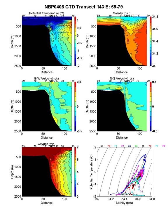
Ross Sea. But given the general properties of bottom water
in the Australian-Antarctic Basin, HSSW may not be a significant contributor in
this sector, much less to the global ocean. Deep water modification in this
region is classic Carmack/Killworth large-scale interleaving, as has been noted
previously, a process not often reported in the Ross sector. Waters over the
upper slope were remarkably fresh, even in comparison to summer measurements.
Modified Circumpolar Deep Water (MCDW) intrusions onto the shelf seemed
relatively weak and shallow, and a tendency is noted for deep water and shelf
water to enter/exit the shelf across or near the same sills. Of course that
traffic keeps appropriately to the left, this being the southern hemisphere,
and may also be evidenced by bottom temperature distributions on the slope.
Shelf water formation was ongoing, albeit intermittently (see VMP section
below), and we are increasingly convinced, as others may already know, that the
smaller, less-heralded coastal polynyas, initially neglected in favor of the
storied Mertz, are where the saltiest shelf water is formed. Ice Shelf Water
(ISW) was also observed, but must compete with the effects of strong surface
forcing in winter, and may be less apparent thereby. On A-3 Leg 2, we began by occupying shallow,
widely-spaced reference CTD stations across the eastern Ross Gyre, while moving
southward through the pack near the prime meridian. Just prior to that time,
satellite data suggested lower ice concentrations might be encountered across
the eastern end of the Gyre, but that seemed like a long and potentially risky
route to reach the AnSlope mooring sites. A substantial flaw lead north and
slightly west of Cape Adare had beckoned for weeks, and appeared to be located
near the shelf break, so we diverted SW toward it, across the Adare Trough. At
that point we began to encounter much thicker, more compact ice, and had barely
reached the downslope end of a planned transect when a large storm halted the
proceedings. Persistent easterlies closed off the flaw lead and then strong SE
winds moved us much farther NW than desired. Much fuel was consumed backing and
ramming toward the SE before we were finally able to accomplish a transect
across the 'Visbeck' mooring (Figure 2). Ice and weather conditions then
improved and remained good for the rest of our Ross Sea survey. Several
sections were completed in the vicinity of the Drygalski Trough sill, one near
the AnSlope moorings. VMP profiling near the Drygalski sill was followed by a
section downstream and across the outer Joides Trough, and along the outer
western axis of the Challenger Trough. By then it was time to begin heading north,
and along that route short sections were occupied across the slope and outer
Iselin Bank, ending with a deep cast at the northern side of a passage north of
the Bank. On both legs of the cruise, XBT casts were utilized along some
transects to guide station work, add detail to the lateral thermal structure,
and save time. The Ross sector was also found to be fresher than anticipated
at this time of year, with the ASF more than a spring tidal excursion south
of the continental shelf break. Both east and west of Iselin Bank, bottom water
on the continental slopes indicated a fresh shelf water/surface water component,
quite likely derived from the E-W flow that tracks the ASF. ISW continues to
elude us on the slope, implying that little of it leaves the shelf in undiluted
form, most of it recirculates back under the Ross Ice Shelf, or we have yet
to stumble on its primary exit time/location during brief surveys. The apparent
weak roles of
Figure 2.
Transect across the outer shelf
and slope near 173°E (Figure A-2). Panels show potential temperature,
salinity, zonal velocity, meridonal velocity, and dissolved oxygen and a θ-S
diagram. Zonal and meridional velocities have had their means removed. Dissolved
oxygen has been corrected according to the onboard calibration. Conversely, deep water and its
derivative intrusions onto the shelf were alive and well, dominating much of
the subsurface water column and often extending to the sea floor. Has the HSSW
reservoir shrunk to a point where it can no longer keep the MCDW/CDW at bay?
Are we witnessing a response to the anomalous sea ice and glacial ice
conditions over the shelf during recent summers? Were the A-3 measurements
obtained at a time when the forcing was weak and the ocean regime was relaxing
after a more active period caused by the large storm? We trust that the
moorings, when recovered in January 2005 and analyzed in conjunction with the
meteorological and sea ice data, will shed additional light on these issues. The following sections in this
report provide more detail about the profiling, water sampling and underway
observations made on A-3. Most all CTD stations were sampled for CFC, dissolved
oxygen and salinity, vs. 58% and 44% on A-1 and A-2, respectively. Relatively
few helium, tritium and oxygen isotope samples were taken on station, but many
more nutrient samples in order to accommodate onboard processing by the CLIMA
group. Many more XBT casts were also made on A-3, mostly enroute to and from
the study areas, and the accompanying underway sampling was not done on prior AnSlope
cruises (see Section 2.9). As the station table (Table A-1) in the appendix
demonstrates, about 12 days were spent in each of the two study areas, out of
about 55 days at sea and another 5 days in port. Future inspection of RPSC
records will show the NBP 'sailing for science' more than 90% of the time
during A-3. However, when actual time on site is closer to 40%, it may be time
for another rubric to monitor NBP performance. We thank the many people who have contributed in
many ways to the AnSlope 3 adventure, aka NBP04-08. From the responsive and
responsible ECO/RPS hands, to the conscientious and congenial science party,
all have persevered with talent, care and good humor. We also thank OPP
O125172, for which we have tried to give good weight in return. We may have
spurned Hobart and ranted at Holik,
but from Denver to Palisades, Seattle to Suitland, McMurdo to Timaru,
many others have helped to see us through. From a perfect storm off Cape Adare to a perfect finish
across the ACC, from here to there and back again, we now have some icy tales
to tell. Science Staff Stan Jacobs Chief Scientist LDEO Gerd Krahmann LADCP/CTD/tracer sampling LDEO Robin Robertson CTD/XBT/underway sampling LDEO Deb LeBel CFC sampling/analysis LDEO Guy Mathieu CFC sampling/analysis LDEO Raul Guerrero CTD/autosal/sample analysis LDEO/INIDEP Sarah Searson CTD/XBT/underway sampling LDEO Alison Criscitiello Oxygen/tracer sampling LDEO Basil Stanton Oxygen/sampling analysis LDEO/NIWA Laurie Padman VMP/ AnSlope PI/ Earth & Space Research Loren Mueller VMP/CTD/XBT Earth & Space Research Denis Franklin Sea ice observations LDEO Ian Southey Sea ice/ sea bird observations LDEO Sarah Dolman Marine mammal observations IWC/ WDCS Kelly Asmus Marine mammal observations IWC/ Deacon University Alessandra Campanelli nutrient sampling CLIMA/ ISMAR-CNR Serena Massolo nutrient sampling CLIMA/ Universitá di Genova RSPC Support Staff Karl Newyear Marine Projects Coordinator Annie Coward Marine Technician Amy West Marine Technician Jeff Morin Marine Science Technician Sheldon Blackman Electronics Technician Kevin Pedigo Electronics Technician Rob Hodnet Information Technician Dean Klein Information Technician LDEO = Lamont-Doherty Earth
Observatory CLIMA = Climate Long-term
Interaction of the Mass balance of Antarctica (Italy) INIDEP = National Institute
for Fishery Research (Argentina) IWC = International Whaling
Commission NIWA = National Institute
for Water and Atmospheric Research (New
Zealand) WDCS = Whale and Dolphin
Conservation Society Temperature, salinity, and dissolved oxygen
profiles were obtained with a SeaBird Electronics SBE 911+ CTD system fitted
with 2 sets of ducted conductivity-temperature sensors, dual pumps, and one/two
SBE 43 dissolved oxygen sensors. The sensor suite was mounted vertically on a
flat surface just inboard of the lower CTD/rosette frame supports. As the
sensor pairs gave slightly different values and drifted slightly with time (sea
section 2.4.), post-cruise calibration plus intercomparisons with bottle data
will be required during data reduction. A transmissometer and fluorometer were
also installed, both with 6000 m-depth capability. One Hertz GPS data from the
vessel's Ashtech GPS was merged with the CTD data stream and recorded at every
CTD scan. Data were acquired using a PC running Windows 98 and SeaBird's Seasave
software, version 5.30b. Raw data were copied over the network to a separate
drive immediately after station completion. Processed data were copied to a
network disk drive and were generally available within minutes after station
completion. Spiking and modulo error counts were of
increasing concern during the first leg of the cruise, and led to analyses
suggesting a conducting cable fault in the vicinity of 600 m. After
considerable discussion, the outer 700 m of cable was lopped off after station
79, enroute to Timaru, followed by a new end termination and test cast near the
end of XBT transect #2 (station 80). These measures did not totally eliminate
either the spikes or modulo errors, but reduced them to insignificant levels
during the 2nd leg. Station 57 needed to be restarted due to pump tubing
problems. At station 98, the pump hose for the primary sensors was dislodged
when bottles were fired. Consequently, data values for station 98 subsequent to
47 db are suspect. The pump for the secondary sensors was found to be
operating incorrectly at the start of station 132 and was replaced. Most profiles reached within 10 m of the sea
floor, with bottom approach guided by a 12 kHz pinger (OSI) mounted on the
frame, along with an SBE bottom contact switch fitted with a 10 m lanyard and
weight. The pinger and bottom contact switch generally worked well, except for
a few stations where the ship drifted rapidly and/or the bottom current was
strong, or where the ship's thrusters complicated the bottom approach. (See
section 2.11 below.) Transmissometer readings were nearly constant for all
casts except # 85, which is puzzling, since early data in this region indicated
significant suspended material near the bottom. In an attempt to determine
whether the instruments might be at fault, transmissometers were switched in
and out before various casts (20, 29, and 81) and the transmissometer cable was
changed (cast 9). The surface reference marker on the CTD cable indicated the
depth of the CTD beneath the surface was changed before casts 5 and 80. Water samples were taken with a 24-position SBE
32 Carousel sampler with 10 liter 'Bullister' bottles. Water was collected for
onboard analyses of salinity, dissolved oxygen, chlorofluorocarbons (CFCs) and
nutrients (silicate, phosphate and nitrate). Salinity and oxygen analyses are
primarily for standardizing the CTD conductivity and O2 sensors.
Additional samples were drawn on some stations for later analysis at LDEO and
in Italy of helium, tritium,
oxygen isotopes and nutrients. The rosette was generally trouble free except
for minor problems such as trip failure due to sticky latches, open vents and
dislodged O-rings, as noted on the bottle cop sheets. Most bottles were closed
on most stations, but usually two or more were fired at each chosen depth, as
the water columns encountered rarely required more detailed sampling. Sample
depths emphasized water column extrema in T and S, regions with homogeneous
layers for salt and O2 control, and layers near the sea surface and
sea floor. Several experiments were conducted with tripping procedures, such
as cycling already closed bottles to greater depths on yo-yo stations, and
tripping during the upcast without stopping. The fish was typically raised and
lowered near 50m/min, but slower near the air and sediment interfaces. Station setup was more problematic than we
encountered on prior NBP cruises, often requiring more than 30 minutes from the
time a decision was made to stop for station until the ship was ready for the
CTD to be launched. This complicated related preparations, such as starting
the LADCP system, and on one occasion an LADCP connector was deep fried as the
package went over minus its dummy plug. Time required to get the CTD out of the
water and back into the relative warmth of the Baltic room was also of concern,
given –20oC air temperatures at some stations. While the CTD sensors
seemed to withstand such thermal shock without incident, we cannot easily
account for all jumps that occurred, e.g. between sensor output and bottle
oxygen values. On the other hand, some time was saved by limiting the O2
sensor equilibration time at 4 m depth to 1-2 minutes prior to each station. We
do not believe this negatively impacted O2 sensor performance, which
was less good overall than expected from these new instruments. After rather
large offsets and jumps during leg 1, a second O2 sensor was added,
beginning at station 88, with some improvement. Hysteresis also continues to
plague these sensors, although much less so that the earlier Beckmann oxygen
units. See section 2.5 for more details on the bottle-CTD oxygen comparisons. Against some prior advice, and after a full
round-house discussion, the Baltic room was made available for VMP casts rather
than undertaking that operation on deck and in the wet lab. To protect the CTD
during the 12-24 hr VMP stations, during which time the Baltic room door was
open, the CTD/rosette was shunted aside, but not disconnected from the
conducting cable. It was covered with a tarp, kept warm by a small heater and
the sensors were drained. This procedure worked reasonably well, although water
was left on the sensors during the last VMP cycle, and a heater may have
failed, perhaps accounting for a coincident shift in the secondary conductivity
sensor output (see section 2.4.). As noted above, all the CTD temperature,
salinity and oxygen data will be reprocessed after post-cruise sensor
calibration data are available. At that time it will be determined whether the
primary or secondary sensor outputs, or some combination of the two, will be
used for the final data set. [Stan Jacobs] A dual head (one up and one
downward looking) lowered ADCP (LADCP) system was attached to the CTD/rosette
for the entire cruise. Three different heads were used. All units were versions
of the 300kHz “workhorse” type. During leg one to the George V Coast, the
upward looking system (SN 5254) was a loan from RDI, the ADCP manufacturer manufacturer,
while the downward looking was the most reliable unit owned by Lamont (SN 149).
SN 5254 is a newly developed head with a stronger output power. RDI thereby
hopes to extend the range of the workhorses under difficult conditions such as
the low amount of scatterers in parts of the deep ocean. During test station 1 the battery
case developed a leak through which sea water came in contact with the battery
pack. This was not noticed directly after the cast. A few days later (there was
a 5 day gap between the test and the second station) it was found that one endcaps
of the battery case had been blown off. It was not clear whether the alkaline
batteries exploded themselves or whether electrolysis caused the failure of the
endcap assembly. As the battery case was heavily corroded a spare battery
housing was prepared and installed. During the first few stations unit
SN 5254 developed one bad beam. As the RDI workhorse systems each have four
transducers they can still operate with one failing transducer. Only the error
estimate of the velocities is lost in this case. Unfortunately this system
developed a second failing transducer, which rendered it inoperable. Also, we
did not find that 5254 provided a significantly longer range. After cast 12,
when the second transducer failed, we removed both systems from the rosette. The data gathered until then was of
reasonable acoustic quality at most stations. All profiles in the George V
Coast region were, however, plagued by the close proximity to the south
magnetic pole. In this region the flux gate compass from which the ADCPs derive
their heading does not work reliably. During the first leg of the cruise an
attempt was made to derive ADCP heading from other data. So far we have not
been able to create a method of recovering the heading over the full length of
a profile. Under some circumstances the developed algorithm, which is based on
the assumption that the current measured by the ADCP does not change much over
the 1.5 second ping interval, is able to recover parts of the rotation. In
these cases it is possible to compare the flux gate measured heading with the
independently derived rotation and evaluate the quality of the measured
heading. In a few cases this evaluation indicated that the measured heading was
reliable in spite of the proximity to the south magnetic pole. After e-mail consultation with
colleagues at LDEO we resumed LADCP operations at station 49 with SN 150 as the
upward looking unit. Except for the unusable compass data both profilers worked
well. Before station 58, the dummy plug
was not placed on the CTD/rosette side of the connection between ADCPs and
computer. One of the power holding pins of the plug corroded away during the
cast. This rendered unusable the second quintopus cable, which connects the battery
with the two ADCPs and the deck cable. The first had been found early during
the cruise to be unreliable. ET Sheldon Blackman cut the corroded part off the
second cable and replaced it by the same part of the uncorroded, but
unreliable, first cable. He built a high pressure safe connection between the
two salvaged pieces. A replacement cable ordered from the manufacturer did not
reach the ship in time for our mid-cruise port call in Timaru, NZ. A new
battery housing was received but has not been used. During the second leg of the cruise
no serious problems were encountered. SN 149 developed one broken beam but
remained otherwise fully functional. Previous experience with LADCP
systems in the Southern Ocean indicated that profiles going deeper than about
1500m give unreliable results as the amount of scatterers at these depths is
too low for the RDI workhorses. Several such profiles lead to suspicious
looking results. All in all, about 50 out of 100
LADCP profiles were located far enough from the magnetic south pole and shallow
enough for a sufficient amount of scatterers. Table A-2 in the appendix lists
the LADCP profiles taken and whether they are deemed reliable Figure 3: Example LADCP profile showing a three layered
current structure. after being processed with the current version of the
processing routines (see Figure 3 for a profile deemed reliable). As the
processing routines are under continuous development, we always hope that
future advances will result in additional reliable results. [Gerd Krahmann] Operations Summary The Vertical Microstructure
Profiler (VMP, a.k.a. “Vampire”; see photo on Figure 4) is a tethered,
free-fall profiler measuring microscale (order 1 cm) temperature and
conductivity (T and C), and velocity shears ¶u/¶z
and ¶v/¶z. Vampire also carries pumped calibrated CTD-quality T
and C sensors (SeaBird SBE-3 and SBE-4), for providing simultaneous
high-accuracy (but lower vertical resolution) scalar data. Instrument depth and
motion (speed and tilt) are monitored by a pressure sensor and 3‑axis
accelerometer. The latter data provide a means for removing instrument-induced
“noise” from the shear sensors. The instrument fall speed w is
~0.6 m/s, the rate determined by a balance by syntactic foam buoyancy
elements and a “chimney sweep” drag brush. The chosen fall speed is a
compromise between sensitivity of the shear probes (µ w2: i.e., better at higher w) and the
vertical resolution of the microscale scalar sensors (better at lower w).
Vampire is ~2.2 m long when fully assembled. The primary goal of deploying
Vampire on AnSlope-3 was to obtain higher-quality measurements of turbulent
mixing rates than we obtained on AnSlope-1 using the CTD-mounted Microstructure
Profiling System (CMiPS). In particular, we hoped to obtain turbulence data
through the upper interface of the bottom-trapped plumes of outflowing dense
shelf water, as seen in AnSlope 1 CTD/LADCP/CMiPS data. Vampire was deployed from the
Baltic Room, replacing the CTD there for periods of a few hours to a day. Once
the technique for converting the Baltic Room was sorted out, turnover took
about 2 hours to set up for Vampire, and 1.5 hours to return to CTD operations.
Maximum deployment depth was ~800
m. We had ~1300 m of cable available on the winch drum, and could have
deployed deeper if there had been a good scientific justification. However,
because Vampire “kites” with the drag on the cable due to the lateral motion of
the ship (generally tied to wind-driven ice motion) relative to the deep ocean
currents, the amount of line that must be unspooled from the winch is generally
greater than the instrument’s final depth. Thus, we tentatively estimate a
maximum profiling depth of ~1000 m for the present winch cable. Mechanical Issues The main technical problem we
encountered with Vampire deployment was with the winch drum. This drum was
re-engineered from a standard commercial model in order to accommodate more
cable (for deeper profiling). However, the drum flanges were not strong enough
to support the pressure exerted by the cable during retrieval: as a result, the
drum flanges were warped, and subsequently rubbed against the supporting winch
frame. Data Storage Vampire data are included on the
Cruise CD. The data are provided in Matlab format, and are listed as “raw_data”
and “processed_level_1”. The raw-data files are in counts (digitized voltages
and frequencies) as originally recorded directly off Vampire. The
process-level_1 files are a quick-look version of data in engineering units.
These data require further post-processing, but contain versions of all the
signals that are useful to look at. Setup files (*.setup; ASCII text), list
basic information about configuration for each deployment. Each file contains header
and data structure arrays (HDR and DATA). See Matlab documentation for how to
access contents of structure arrays. HDR data are profile start time, time
base (always UTC here) and the limits used for trimming bad data off the start
and end of the original data files (using “trim_files.m”). DATA arrays are in
two forms, “fast data” and “slow data”. For the first two deployments in AnSlope
3, the fast and slow sampling rates were 512 Hz and 64 Hz, respectively. For
reasons explained below, these rates were reduced to 256 Hz and 32 Hz for
the third deployment. Table 1 shows signals in the DATA structure array.
Information in structure arrays is accessed as follows: load A3_001_030.mat; % load
process_level_1 file, giving HDR and DATA % structure
arrays Pf = DATA.P_fast; % etc. Variable Units Sample rate Description Ax, Ay, Az m s-2 Fast 3-axis accelerometer tilt degrees Fast Derived from Ax, Ay, Az P_fast Dbar Fast Pressure record for fast channels P_slow Dbar Slow Pressure record for slow channels W m s-1 Fast Fall speed Sh1, Sh2 s-1 Fast Velocity shear from airfoil probes T_SBE oC Slow SBE-3 temperature C_SBE Slow SBE-4 conductivity S_SBE psu Slow Salinity from T_SBE and C_SBE t_f s Fast Time (seconds) for fast channels t_s s Slow Time (seconds) for slow channels T1_lo oC Fast FP07 T1 low-resolution T1_hi oC Fast FP07 T1 pre-emphasized (high-res) dT1dz oC m-1 Fast FP07 T1 gradient T2_lo oC Fast FP07 T2 low-resolution T2_hi oC Fast FP07 T2 pre-emphasized (high-res) dT2dz oC m-1 Fast FP07 T2 gradient C_raw 1 Fast Raw output for C_dC 1 Microconductivity not available on AnSlope
3. Table 1:
Parameters sampled by Vampire, and their sampling rate categories. Results A total of 60 good profiles were
obtained in 3 sessions as described below (see also Table 2, below). One
profile is shown in Figure 4. Graphical summaries of all processed_level_1
profiles are on the cruise CD/DVD as *.PNG graphics files. Deployment 1: Intrusions along the George V
Land Coast shelf break Vampire was deployed for a period of ~20 hours in
sea ice over the upper slope in the George V Land region (AnSlope 3, first
leg). 22 profiles were obtained in this period. The ship generally drifted
with the ice, with one repositioning (after profile A3_001_012) to move the
ship up the slope closer to the shelf break. The data set provides information
on the turbulence associated with interleaving intrusions of cold shelf water
and warm offshore water of CDW origin. The number of intrusive layers
frequently corresponded to the number of high-backscatter layers visible in the
38 kHz Ocean Surveyor vessel-mounted ADCP. There are a few potential
explanations for this observation, ranging from the two water types (“shelf”
and “offshore”) having distinct scatterer populations, to the higher
backscatter that is expected theoretically, associated with high variance of
high-wavenumber thermal (and hence sound speed) gradients. Deployment 2: Upper-ocean response after katabatic winds
in the Mertz Polynya Vampire was deployed for a period
of ~6 hours in the open water of the coastal polynya along the edge of the
Mertz Glacier Tongue. 10 profiles were obtained in this period. The ship used
dynamic positioning (“DP”) to stay in an exact location and with a consistent
orientation to the wind. Deployment was initiated during a period of intense
offshore katabatic winds, with speeds of 50-60 knots, and clear visual evidence
of rapid surface cooling and ice formation. Unfortunately for our science
interests, the wind dropped to ~10 knots during the ~2-h taken to convert the
Baltic Room to Vampire use. However, the air temperature remained cold, below
-10oC. The data set provides some information on the turbulence energetics
of the surface mixed layer under moderate convective conditions, but we were
frustrated at being so close to a “katabatic” data set and missing it.
Nevertheless, from preceding CTD operations in the harsh conditions, it is
clear that the ship is capable of operating (with CTD or Vampire from the
Baltic Room) in high-wind, ice-free, high-convection conditions using DP rather
than free drift. Vampire was deployed for a period
of ~24 hours in sea ice over the sill at the northern end of the Drygalski
Trough. 28 profiles were obtained in this period. Winds were light, and the
ship drifted in a rough ellipse presumably driven by ocean tidal currents and
perhaps some near-inertial (wind-forced) variability. The data provide
information about mixing between an intrusion of Modified Circumpolar Deep
Water (MCDW) and the cold surface layer and cold, dense bottom layer. A sample
profile from this deployment (A3_002_023) is shown below (Figure 4). We experienced two problems during
this station. First, upon original setup, the data acquisition system reported
many “Bad Buffers”, symptomatic of noisy or erratic communication with the
instrument. After consulting the manufacturer over Iridium phone, we lowered
the communication baud rate and instrument sampling rate (the latter from 512
Hz to 256 Hz). This did not solve the problem, and the cause of the
signal noise was ultimately determined to be the deck cable leading to the
winch. The entire data set was acquired, however, at the lower sampling rate.
The second problem was that we accidentally bottom-crashed Vampire after drop
A3_002_012, breaking the microstructure sensors. The crash occurred because of
the way Vampire is deployed: in order to obtain good data, cable is let out
faster than the instrument falls, so that the real-time displayed pressure at
Vampire is not a good indication of how deep the instrument will ultimately
fall. We need to mark the wire accurately, and also monitor ship-recorded water
depth more carefully. Displays of depth from the Bathy-2000 (“BAT”) system
are in “uncorrected meters”, i.e., based on a sound speed of 1500 m s-1.
For accurate approaches towards the seabed, we also need to account for the ~1%
difference between depth (in m) and pressure (in dbar). The data from this deployment show a strong
modulation of mixing rates in the MCDW intrusion during the day. Data were
collected just after neap tides for this region; nevertheless, it is likely
that mixing rates are influenced by variations of the predominantly diurnal
tidal currents during the course of a day. We were not able to test the
variability in mixing between spring and neap tides, but we take the present
data set as indicating that tides are an important contributor to mixing of
MCDW intrusions and dense shelf water in the northern trough and over the sill.
This is a potentially significant preconditioning mechanism for determining the
average volume and density of shelf water exiting the NW Ross Sea troughs. Acknowledgments A large number of people contributed to Vampire
operations on AnSlope 3. We thank Annie Coward and Jeff Morin (RPSC) for
working out the mechanics of how to deploy Vampire from the Baltic Room, and
helping to implement the solution. Amy West and Karl Newyear (RPSC) also
contributed to converting the Baltic Room between CTD and Vampire use. Alison Criscitiello,
Raul Guerrero, Robin Robertson, Sarah Searson and Basil Stanton all helped with
Baltic Room Vampire operations. The ship crew’s ability to keep workable space
around the Baltic Room is gratefully acknowledged. The name “Vampire” was
coined by Robin Robertson just before Halloween. [L. Padman and L. Mueller] Table
2: Details of Vampire profiles during AnSlope 3 Profile ID
Date Time Lat Lon File size
(UTC) (bytes) Deployment
1: George V Land Shelf Break A3_001_010.mat
25-Oct-2004 13:18:34 -65.922 144.602 19289784 A3_001_011.mat
25-Oct-2004 13:44:52 -65.921 144.606 53301784 A3_001_012.mat
25-Oct-2004 14:47:58 -65.918 144.616 78382784 A3_001_013.mat
25-Oct-2004 15:41:20 -65.916 144.624 79766784 A3_001_014.mat
25-Oct-2004 16:51:04 -65.913 144.635 84837784 A3_001_015.mat
25-Oct-2004 17:51:54 -65.911 144.643 82993784
Moved South 2.5 km, A3_001_016.mat 25-Oct-2004 21:27:52 -65.935 144.654 66272784 up-slope towards A3_001_017.mat
25-Oct-2004 22:24:42 -65.936 144.659 74017784 shelf break A3_001_018.mat
25-Oct-2004 23:43:30 -65.937 144.661 76313784 A3_001_019.mat
26-Oct-2004 00:19:38 -65.937 144.661 74017784 A3_001_020.mat
26-Oct-2004 01:12:54 -65.937 144.660 53792784 A3_001_022.mat
26-Oct-2004 01:18:34 -65.938 144.660 19161784 A3_001_023.mat
26-Oct-2004 02:18:48 -65.938 144.656 68280784 A3_001_025.mat
26-Oct-2004 03:20:46 -65.937 144.650 69509784 A3_001_027.mat
26-Oct-2004 05:07:34 -65.937 144.614 61323784 A3_001_028.mat
26-Oct-2004 06:11:34 -65.936 144.599 59888784 A3_001_029.mat
26-Oct-2004 07:08:18 -65.936 144.582 60821784 A3_001_030.mat
26-Oct-2004 07:38:44 -65.936 144.573 10981784 A3_001_031.mat
26-Oct-2004 07:45:16 -65.936 144.570 14427784 A3_001_032.mat
26-Oct-2004 08:03:46 -65.937 144.564 47645784 A3_001_033.mat
26-Oct-2004 08:34:52 -65.937 144.553 53362784 A3_001_034.mat
26-Oct-2004 09:08:28 -65.937 144.539 47901784 Deployment
2: Mertz Polynya A3_001_035.mat
29-Oct-2004 03:44:58 -67.056 145.178 76785032 A3_001_036.mat
29-Oct-2004 04:21:40 -67.056 145.178 56528024 A3_001_037.mat
29-Oct-2004 04:51:22 -67.056 145.178 53153888 A3_001_038.mat
29-Oct-2004 05:22:44 -67.056 145.178 44035288 A3_001_041.mat
29-Oct-2004 06:36:34 -67.056 145.178 44087104 A3_001_042.mat
29-Oct-2004 06:58:48 -67.056 145.178 44867392 A3_001_043.mat
29-Oct-2004 07:29:44 -67.056 145.178 41162040 A3_001_044.mat
29-Oct-2004 07:52:14 -67.056 145.178 39350512 A3_001_045.mat
29-Oct-2004 08:14:08 -67.056 145.178 33438408 A3_001_046.mat
29-Oct-2004 08:44:00 -67.056 145.178 79168568 Deployment
3: Drygalski Trough Sill A3_002_002.mat
22-Nov-2004 19:32:08 -72.216 172.960 15928664 A3_002_003.mat
22-Nov-2004 20:19:56 -72.222 172.967 27171720 A3_002_004.mat
22-Nov-2004 21:06:08 -72.229 172.976 22909704 A3_002_010.mat
22-Nov-2004 22:13:44 -72.234 172.993 27233696 A3_002_011.mat
22-Nov-2004 23:11:44 -72.238 173.006 27171720 A3_002_012.mat
22-Nov-2004 23:59:30 -72.240 173.018 26078504 Bottom-crash A3_002_014.mat
23-Nov-2004 01:33:38 -72.248 173.040 26421912 A3_002_015.mat
23-Nov-2004 02:18:56 -72.251 173.051 29440448 A3_002_016.mat
23-Nov-2004 03:20:24 -72.255 173.067 29441464 A3_002_017.mat
23-Nov-2004 04:06:08 -72.255 173.082 25953536 A3_002_018.mat
23-Nov-2004 04:50:08 -72.255 173.095 27015256 A3_002_019.mat
23-Nov-2004 05:38:06 -72.257 173.110 28514872 A3_002_020.mat
23-Nov-2004 06:24:50 -72.257 173.128 26016528 A3_002_021.mat
23-Nov-2004 07:15:16 -72.255 173.147 32428504 A3_002_022.mat
23-Nov-2004 08:05:56 -72.254 173.167 28483376 A3_002_023.mat
23-Nov-2004 08:49:56 -72.251 173.183 26859808 A3_002_024.mat
23-Nov-2004 09:33:32 -72.248 173.196 25828568 A3_002_026.mat
23-Nov-2004 10:50:10 -72.240 173.205 27952008 A3_002_028.mat
23-Nov-2004 11:38:48 -72.236 173.205 27889472 A3_002_029.mat
23-Nov-2004 12:29:08 -72.231 173.199 28763144 A3_002_030.mat
23-Nov-2004 13:16:20 -72.228 173.191 29766280 A3_002_031.mat
23-Nov-2004 14:06:16 -72.227 173.181 28170448 A3_002_032.mat
23-Nov-2004 14:43:20 -72.227 173.174 27358664 A3_002_033.mat
23-Nov-2004 15:28:58 -72.228 173.164 26640352 A3_002_034.mat
23-Nov-2004 16:14:06 -72.230 173.155 26140480 A3_002_036.mat
23-Nov-2004 17:01:40 -72.235 173.148 26140480 A3_002_037.mat
23-Nov-2004 17:58:50 -72.241 173.143 28295416 A3_002_038.mat
23-Nov-2004 19:02:16 -72.248 173.143 29357136 In order to monitor the performance of the CTD
conductivity sensors, 818 salinity samples were analyzed using the on-board autosals.
Autosal SN 59-213 was used for stations 1 to 88 (518 samples), while stations
91 to 142 were measured on Autosal SN 61-670 (300 samples). Both instruments
performed within factory specifications, although instrument 59-213 required
lowering the flow rate to obtain adequate repeatability. Laboratory temperature
control was excellent, remaining 1 to 2ºC below the setting temperature (24ºC).
The fan set up on top of one of the salinometers kept the lab temperature
vertically homogeneous. Data from the Autosals were captured using the ACI
2000 hard/software package. The connection failed on 3 occasions, but without a
clear pattern, we were unable determine the cause. This occurred with both autosals,
using the ACI and a home made box (probably from SCRIPP’s), and two 50 way
ribbon cables. ACI did not reply to email inquiries concerning this problem. An average of two boxes (48
samples) was measured on each “run” with standardization performed at the
beginning and end of each. The standards for calibration came primarily from
batch P140 (OSI) from November 2000 (approx. 44 vials) plus three P141 vials
from June 2002 and two P143 vials from February 2003, for inter-calibration.
On three occasions (Runs 3, 16 & 19), vials from two different batches were
used consecutively without finding differences between them. As seen in Table
3, little or no re-standardizing was required between runs. The Standby reading
for instrument 213 ranged from 6135 to 6141 while instrument 670 varied from
6067 to 6072. For reference, 5 units change in the Standby readings is
equivalent to .00005 CR units or about 0.001 psu. Errors in salinity resulting from
the primary and secondary conductivity sensors were tracked throughout the 142
stations (Figure 5). Salinity errors, denoted DeltaS, are reported as rosette
salinity minus CTD salinity. The primary conductivity sensor showed a stable
bias from station 1 throughout station 133. Mean Delta S was -0.0015 with a
standard deviation of 0.0022. For the estimation of this error, 655 points out
of 761 (86 %) were used. Points excluded were greater than 1.5 times the
standard deviation of the mean error. The secondary sensor started with a DeltaS
@ +0.0075 and decreased down to near 0
around station 50. As this sensor’s DeltaS is neither constant nor linear, it
may not be as suitable as the primary for final calibration. Both sensors
appear to drift from station 134 to 138 and from station 139 to 142 the offsets
are constant at much higher DeltaS values (+0.010 for the Primary and +0.0044
for the Secondary). 1 2 3 4 5 6 7 8 9 10 11 12 213 6139 6139 6138 6138 6141 6137 6138 6135 6140 6141 6137 6138 Run 13 14 15 16 17 18 19 20 670 6069 6072 6071 6071 6071 6069 6068 6067 Table 3: Salinometer
Standby readings throughout the cruise. Good stability was observed between
runs as little or no re-standardizing was needed. Applying a linear correction as a
function of ‘Sta#’ for 134-138 and a constant offset +0.010 for 139-142, the
residual has a standard deviation of 0.0022. Comparison among Primary and Secondary CTD sensors Differences between the T sensors
(Pri-Sec) are constant around -0.001 throughout the cruise. Differences in S
between the conductivity sensors are more complicated, and include the
following features: - A gradual drift toward
near zero on the secondary sensor from station 1 to 52 (Figure 6). -
A jump (probably in the secondary
sensor) between stations 80 and 81, coincident with the Timaru port call, in
spite of the fact that both sensors were flushed and kept filled with DI water
at that time. The aft dry lab distiller, that provided DI water for the
sensors, was out of service. Sensors were flushed after each station only with
filtered water. - The anomalies at
station 98 were caused when the primary hose was knocked off when a bottle was
fired at 47 db. - A jump between
stations 110 and 111 (not obvious in DeltaS from the bottles) occurred at the
time of a VMP station staged from the Baltic room. With the door open, the CTD
package was covered and TC sensors were warmed by a heater. However, on this
occasion, the TC plumbing was left with filtered water on, the heater was found
off and water in the plumbing was slushy. - Station 111 shows a
larger S0-S1 than typical, and a result from tripping bottles while the CTD was
underway. From station 134 to 138 the
difference between primary and secondary drifts, as observed in both sensors
when compared against bottle salinities. However, the primary sensor showed a
steeper drift than the primary. The cause of this drift is unknown, but could
be oil or biological coating/stain on the electrodes that may change their
geometry. It could also be a problem within the CTD. SBE technical services
might be consulted to check out, which could require factory service. - From station 139 to
142 the difference between primary and secondary sensors returned to a constant
value, but much higher than before. Both sensors then differed from the bottle
data by +0.010 and +0.0044, primary and secondary, respectively. Along XBT sections, thermosalinograph
(TSG) salinities were comparies with samples drawn from the sea surface water
system and analyzed with the Autosal. Out of 111 samples, 109 were used to
estimate the preliminary error of the TSG. The error was constant throughout
the cruise with a mean value of –0.005 psu and a standard deviation of 0.011 psu.
[Raul Guerrero]
A SBE43 dissolved oxygen sensor was
incorporated in the CTD sensor array. At CTD stations water samples were drawn
from selected rosette bottles for dissolved oxygen analysis using the modified
Winkler method. Whole bottle samples were titrated using an amperometric titrator
designed by Dr. C. Langdon. An RPSC titration unit was used while other
laboratory equipment, sample flasks and chemicals were supplied by LDEO. Titrations were done on 865 CTD
samples and 181 surface samples from the 4 Transects between New Zealand and Antarctica.
No major problems were encountered with the oxygen analyses. The usual minor
problems such as bubbles in the micro burette or sticking of bottle top
dispensers occurred occasionally. Initially some difficulty was experienced in
getting stable blank determinations and this may have been due to inconsistent
performance of the 1 ml standard dispenser. However this eventually settled
down and is not thought to have affected O2 results. Sensitivity
analysis of the WHP O2 equation shows that final accuracy is only
very weakly affected by the blank value. Standard determinations showed some
variation but these were within the usual accepted range. Comparison of the rosette O2
and the primary CTD O2 sensor data showed that the sensor was
reading consistently low. The Delta O2 (rosette – CTD) at each station
(color coded for in situ temperature) are shown in Figure 7. Note that the 3
panels in this figure are plotted with some overlap to show the changes over
time. Delta O2 values were typically in the range 04 - 1.2 ml/l, and
the temperature dependence is evident with the largest Delta O2
values at low temperatures. The figure also shows there were variations with
time throughout the cruise. These variations were a slow drift over time
interspersed with periods of apparent stability. On occasions there was an
apparent abrupt change in O2 sensor calibration while on station.
This occurred at Stations #52 and #98 and accounts for the outliers at these
stations. The problems at Station # 98 are covered in the CTD section of the
report. Another outlier at Station #124 has been checked and remains
unexplained. Plotting Delta O2 against
CTD Temperature for all data showed the clear decrease in Delta O2 with
increasing temperature up to a temperature of 2.0, with a generally flat
response at higher temperatures. The All Data plot showed a large spread but
suggested that a simple temperature correction could be found by taking
stations in similar groups suggested by Figure 7. Figure 8 are plots of Delta O2
against temperature for all 142 Stations in 8 groups. For each plot a least
squares straight line has been fitted for the data at temperatures below 2o
C. The straight line parameters and Root Mean Square deviations of Delta O2
from the straight line are given for each panel. We believe these parameters
should be used in the final post processing of the CTD O2 data. An additional SBE43 sensor was
installed on the CTD at Station #88, as a secondary while retaining the
original primary sensor. Comparison of these sensors showed a mean difference
of 0.336 ml/l, with the secondary sensor reading higher than the primary
sensor. Consequently the secondary sensor values were closer to the rosette
data. The standard deviation between the primary and secondary sensors was
0.094 ml/l. The Delta O2 (rosette-secondary sensor) exhibited a
similar tendency to the primary sensor with higher values of Delta O2
at the low temperatures. These Delta O2 data are shown in Figure 9a
with a fitted straight line as was done for the primary sensor. After removal
of the temperature effect, Figure 9b shows a quadratic curve fitted to the
residuals to remove the pressure dependence, while Figure 9c shows the residual
Delta O2 after removal of both temperature and pressure trends. It can be seen
that the remaining variation is very small with a standard deviation of 0.039
ml/l. The surface water samples on the
four transects (see Figure 10) between New Zealand and Antarctica were drawn
from the thermosalinograph sea water system in the wet lab. Some problems were
experienced with fine air bubbles in the water flow and as a result extra care
was needed in taking these samples. Even then on occasion, fine air bubbles
could form (presumably from out gassing) within the flask during the interval
between sampling and titration. When this occurred appropriate comments were
added to the log sheets. [Basil
Stanton] Figure
7: Difference between titrated and CTD-measured dissolved oxygen. The color of
the dots indicates the temperature. Figure 8: Temperature dependency of the dissolved oxygen deviation
between CTD sensor and titrated measurements. Figure 9: Delta O2 variation for the
secondary O2 sensor. Figure 10:
Titrated dissolved oxygen content on XBT transect 3. Water sampling Water samples were collected using
10-l Niskin-type bottles with coated internal springs and baked
o-rings. CFC samples were the first samples taken and were drawn into
100-ml precision ground glass syringes. The syringes were capped with
stainless steel Luerlock caps and stored in a sink filled with uncontaminated
surface seawater. Tension was maintained on the syringe plunger with
rubber bands and the samples were analyzed within 12 hours of collection,
typically less. For most of the cruise, the water bath temperatures were less
than -1.0C, which ameliorated any potential degassing during sample storage. Sampling from the uncontaminated
seawater line Water samples were collected on all
four transits between New Zealand and the ice. On the first two transits,
samples were collected every two hours; on the second two transits every 30o
of latitude. Sampling was simply a matter of inserting the tip of the syringe
into the length of Tygon tubing providing flow to the syringe water bath and
following standard rinse and storage procedures. Data quality statistics (see
Data Quality section) were not significantly different from samples drawn from
the rosette. Water sample analysis From the syringes, the water
samples were injected through a three-way valve into a calibrated glass volume
(approximately 35 cc, calibrated to better than 0.1%). The three-way valve
and the calibrated volume were flushed with sample water prior to taking the
aliquot for analysis. The water in the calibrated volume
was subsequently transferred to a glass stripper chamber where the dissolved
gases were purged with ultra high purity nitrogen, which was also used as the
gas chromatograph carrier gas. The released CFCs were concentrated by
adsorption on a unibeads 2S cold trap at –70°C. Subsequently the trap was
isolated and heated to 100°C. The desorbed gases were then backflushed
into the chromatographic columns using ultra pure nitrogen. Cooling was
accomplished with liquid CO2 and heating was done
electronically. The entire stripping, trapping and GC analysis procedure
was automated with a Shimadzu Chromatopac C-R8A used to control the sequential
steps of the procedure. Air sample collection and
analysis Air samples were drawn from an
interface with the ship's on-board pCO2 measurement system. Aliquots of air
taken from this line for CFC analysis were passed through magnesium perchlorate
to remove water vapor, isolated in a calibrated sample loop, and then analyzed
in the same way as standard gases (see section on calibration). Samples
were only collected when the wind direction was from the bow to avoid
contamination with the ship’s atmosphere. Gas chromatography The CFC analysis system consisted
of a Lamont-built purge and trap system interfaced to a HP 6890 gas
chromatograph which contained a precolumn (stainless steel, 3 foot length,
0.085 inch ID packed with 80-100 mesh Porasil B) and a main column (stainless
steel 5 foot length, 0.085 inch ID packed with 60-80 mesh Carbograph 1AC)
mounted in the GC oven and maintained at a constant temperature of
90°C. The main column was followed by a 0.085 inch ID, 4 inch long
stainless steel column packed with 80-100 mesh mol sieve 5A. This was
mounted outside the GC oven and maintained at 50°C. Its purpose was to
separate CFC-12 from N2O and it was valved out of the gas stream after
CFC-12 eluted. The detector was operated at 260°C. The
chromatographic run required 8 minutes and the total analysis time was 10
minutes per sample. CALIBRATION Procedure The response of the electron capture detector to
different amounts of CFCs was calibrated by filling 10 different sized
calibrated loops attached to a multiport valve with a gas mixture (CFCs in
nitrogen) of known CFC content. Loops were filled individually and after
relaxation to ambient temperature and pressure, the standard gas was
concentrated onto the cold trap and subsequently injected into the gas
chromatograph by the same procedure used for water samples. Calibration
curves were run approximately once a week during the course of the cruise
and one of the standard volume loops was run frequently (at least every other hour) to check for
drifts in the detector’s response between calibration curves. Standard Lamont standard 842 was used
on this cruise. It was calibrated before and after the cruise against an
air standard (Lamont standard 35078) that had been analyzed at R. Weiss’
laboratory. The CFC concentrations on the SIO98 scale for this standard
are: CFC-11: 387.83
pptv CFC-12: 200.49
pptv CFC-113: 105.82
pptv PROBLEMS A high CFC-11 stripper blank (-0.078
t 0.369 pmol/kg, averaging 0.003 pmol/kg) persisted for most of the cruise. We
believe this is due to a small secondary peak overlapping with the CFC-11 peak,
and post-cruise corrections will be made on shore. DATA QUALITY Stripping efficiency Stripping efficiencies were measured approximately
every day throughout the cruise. The overall averages were 99.8% for CFC-11,
99.7% for CFC-12 and 99.3% for CFC-113. The efficiencies for CFC-12 and CFC-113
would be expected to be higher than CFC-11 because of their lower
solubility. However, the CFC-12 and CFC-113 concentrations were lower
than the CFC-11 concentration for the samples used in these determinations and
thus are more sensitive to small uncertainties in blanks. We do not
believe the stripping efficiency is less for CFCs 12 and 113 than for CFC-11
and a correction has not been made for stripping efficiency for any of the
CFCs. Blanks System and stripper blanks were
measured for every 6-8 water samples that were run and are presented in Tables
4 and 5. The stripper blanks averaged about 0.003, 0.007, and 0.010 pmol/kg
for CFCs 11, 12, and 113 respectively. Blank corrections were made by
interpolating between blank determinations made before and after a given
analysis, and variability in blanks had little effect on the data quality. Rosette bottle/sampling blanks
could not be determined for this cruise because CFC-free water was not
sampled. In cruises where we have been able to determine such blanks, they
have been in the range of 0.002 to 0.005 pmol/kg. We have not applied a
correction for bottle/sampling blank to this data set. Precision The precision of the measurements
was monitored throughout the cruise by making replicate measurements. For
atmospheric measurements, 3-6 replicates were measured at each
location. For water measurements duplicate samples were collected at most
stations. The average precisions of the
atmospheric measurements were 1.26%, 1.42%, and 2.44% for CFCs 11, 12 and 113
respectively. Mean mole fractions were 251.7 ppt, 537.66, and 79.88 ppt. The average differences between
duplicates with CFC-11 concentrations greater than 1 pmol/kg were 1.2% for
CFC-11, 0.5% for CFC-12, and 1.7% for CFC-113. The average differences for
concentrations less than 1 pmol/kg were 0.007 pmol/kg for CFC-11, 0.003 pmol/kg
for CFC-12, and 0.003 pmol/kg for CFC-113. Duplicates were drawn on
approximately 80% of the samples taken from the uncontaminated seawater line.
The average reproducibility was 1.1%, 0.7%, and 1.7% for CFC-11, CFC-12, and
CFC-13, respectively. RESULTS Underway Measurements We compared samples
drawn from the surface bottle (~3 m) from six stations with water drawn from
the uncontaminated seawater supply (~7 m) when the CTD was at the surface at
the end of the cast (Table 4). The average difference was 2.23%, 1.26%, and
1.01% for CFC-11, CFC-12, and CFC-113, respectively. These differences are
only slightly larger than the average precisions for Leg I, during which the
comparisons were made. This suggests that underway measurements for CFCs can
provide useful information, assuming an uncontaminated seawater supply of the
same quality as the Palmer's. We completed four transects between New Zealand and
65-70oS. The four transects reflect a change from late winter to
early spring conditions, with the southern ends of CFC-11 (pmol/kg) CFC-12 (pmol/kg) CFC-113 (pmol/kg) CFC-11 Difference (pmol/kg) CFC-12 Difference (pmol/kg) CFC-113 Difference (pmol/kg) Underway 5.492 2.994 0.540 - - - Station 2 5.402 2.923 0.527 1.67 2.43 2.47 Underway 4.997 2.709 0.490 - - - Station 3 4.885 2.687 0.489 2.29 0.82 0.20 Underway 4.469 2.522 0.418 - - - Station 30 4.348 2.468 0.415 2.78 2.19 0.72 Underway 4.675 2.542 0.445 - - - Station 46 4.492 2.504 0.441 4.07 1.52 0.91 Underway 4.600 2.548 0.444 - - - Station 47 4.667 2.557 0.452 1.44 0.35 1.77 Underway 4.662 2.566 0.439 - - - Station 57 4.611 2.572 0.439 1.11 0.23 0 Table 4 CFC
concentrations for six pairs of stations where both surface rosette and
underway samples were collected together and the differences in concentrations
between the samples Transects 1 and 2 occurring off George V Land and
those of Transects 3 and 4 in the Ross Sea. Concentrations at 7 m (Figure 11)
typically reflect the thermal structure. Variations are more weakly correlated
with salinity variations, as expected from the solubility function for CFCs
(Warner and Weiss, 1985). This initially confirmed the plausibility of the
measurements. Highest concentrations were observed between 60oS and
65oS (Figure 11), reflecting a balance between decreasing surface
temperatures and ice cover slowing gas exchange. On all four transects, saturations
decline essentially monotonically between 57oS and 65oS
(Figure 11). Supersaturations were observed north of about 47oS and
are probably due to warming of the surface waters. On Transects 1 and 2
saturations rose to a maximum at the thermal front at 57oS and
decreased again to the south. On Transect 3, no thermal front was observed,
with no associated increase in saturations. Saturations also dropped markedly
south of 65oS on the last two transects, where we observed heavy ice
cover. Saturations of CFC-12 are typically
about 3% higher than CFC-11 and about 9% higher than CFC-113 (Figure 11). This
likely reflects differences in gas exchange rates, which depend on the
molecular weight of the species. [Deborah LeBel] Figure 11. CFC concentrations and saturations for the
three species along the XBT transects. Stations with indications of
possible meltwater were sampled for He, Tritium and 18O. On some
other stations, only 18O was sampled, mainly near the surface and
seafloor. Samples were drawn by A. Criscitiello and G. Krahmann according to
the sampling procedures provided. 48 He channels, 48 Tritium bottles and 147 18O
bottles were filled from CTD/rosette casts and 162 18O samples were
taken underway near the sea surface from the onboard sea water lines. The
tracer samples will be analyzed at LDEO. [Alison Criscitiello] Approximately 1400
nutrient samples were drawn and processed aboard the ship. About 1150 seawater
samples were taken from Niskin bottles on all CTD/rosette stations, the
remainder were taken from the ship underway system during the four XBT
transects between Antarctica
and New Zealand (Table 6). No. Samples Date Underway 1 108 15-20 October 04 Underway 2 67 1-4 November 04 Underway 3 45 7-15 November 04 Underway 4 72 30 November – 5 December 04 CTD George C Land area 595 20-31 October 04 CTD Ross Sea 572 12-30 November 04 Tot. 1459 57 days Table
6. Number of nutrient samples collected during AnSlope-3. Material and
methods: Seawater samples
were filtered using GF/F Whatman filters (0.7 mm) and immediately
stored at -80°C until analysis. Samples were unfrozen using a warm water bath
(35-40°C) in order to bring them to room temperature immediately prior to
analysis. Analyses were
carried out using an Autoanalyzer TRAACS 800, according to the colorimetric method
suggested by Strickland & Parsons (1972). The determination
of nitrate and nitrite uses the procedure whereby nitrate is reduced in nitrite
at pH 8 in a copper-cadmium redactor. The nitrite then reacts under acidic
conditions with sulphanilamide to form a diazo compound that then couples with naftileliendiamina
hydrochloride (NEDD) to form a reddish-purple azo dye that is measured at 550
nm. The determination
of soluble silicate is based on the reduction of a silico molybdate compound in
acid solution to molybdenum blue by ascorbic acid. Oxalic acid is introduced to
the sample to minimize interferences of phosphate. The absorbance is measured
at 660 nm. The determination
of phosphate is based on the colorimetric method in which a blue compound is
formed by the reaction of phosphate, molybdate and antimony followed by
reduction with ascorbic acid. The reduced blue-phospho- molybdenum complex is
read at 880 nm. Data processing
software AACE, designed by Bran and Luebbe, was used during analysis and allowed
us to check standard quality. Duplicate
analyses, involving samples stored with different methods (described below),
were taken at some stations in order to check whether nutrients (in particular,
silicate) were adversely impacted by freezing. In fact, it is well known
that a correct sample storage is particularly important for silicate
determination when silicate content is higher than 50 mM, as in the case of Southern Ocean
water masses. Silicon tends to polymerize when stored frozen and samples must be
allowed to stand at room temperature before analysis. Tests carried on 55
samples showed that there is not any significant
difference among concentrations found in samples analyzed just after sampling
and after frozen storage (differences are < 5%, so very close to method
precision), showing that no systematic error was made. In addition, a small set
of samples (15) were stored in dark, cold conditions (+4°C) for 5 days before
analysis. The concentrations for these samples are very similar to the ones obtained
for those stored in the two previously described ways. Furthermore, we checked our
standard solutions with some other standards made up for intercomparison
purposes. During the cruise
a quality problem with one of the Nanopure systems was detected in the nitrite
and phosphate analyses. The use of Low Nutrient Sea Water (LNSW), brought on
board at the refuelling stop in Timaru, allowed us to run nitrite samples on
board. But problems in phosphate analysis persisted even using LNSW. Reagent
tests and standard intercomparison did not reveal any analytical faults and in
addition, phosphate analysis results were very sensitive to the ship movements.
Since this kind of problem persisted during the whole cruise, it was decided to
process these samples in Italy.
Samples of the standard solutions prepared on board will be shipped to Italy together with the phosphate samples
in order to control the data quality. Furthermore, about 70 samples were
collected from CTD stations at different depths and from the underway system
and they were frozen (-80°C) just after sampling. These samples, together with
standard solutions run on board, will be processed in Italy using a five-channel Autoanalyzer Technicon II. Results will be
compared with the ones obtained on board for intercomparison purposes and will
be used for more sample storage tests. Analysis of the
last samples taken from underway system during the 4th XBT transect
will be finish on board at the end of the transect if sea conditions permit,
otherwise samples will be analysed in Italy. Results: Leg I – George V Land Coast Measurements in
the George V Land Coast area were carried out in early spring (2nd
half of October). During this period in the shelf area, the water column
exhibited only small ranges of temperature, salinity and nutrients, suggesting
that the water column was well mixed. In fact no vertical trend can be
identified in nutrient concentrations, which range from 70 to 90 mM and from
25 to 29 mM for silicate and nitrate respectively. In the surface
layer low temperature and relatively high salinity indicate that the melting
process is not pronounced, and as a result nutrient concentrations are
relatively high at 69.1 ±10.5 mM for silicate and 26.8±2.2 mM for
nitrate. At the slope area
we can observe the CDW intrusion on to the shelf at depths greater than 200 m.
This water mass can be identified not only from its physical characteristics, Figure 13. Vertical
profiles of temperature (°C), salinity, nitrate (mM) and silicate (mM) in casts
121-127 (Ross Sea). but it can be traced also by high nutrient
concentrations. In particular, silicate is a good tracer for this water mass
,which is characterized by concentrations ranging between 80 mM and 127 mM (99.3±11.3
mM as mean value), but the silicate maximum can often be found a few
hundred meters below the temperature maximum, as already observed by other
authors (Gordon et al., 2000). Nitrate shows a distribution more
homogeneous than silicate also in the slope area, with the highest values
(about 30 mM) coincident with the temperature maximum. “NO“ mean level of
473±22 mM was calculated for CDW at the temperature maximum; this value
falls in the same range as those calculated for the Weddell
Sea (Lindegren&Anderson, 1991) As an example,
Figure 12 shows vertical profiles of temperature (°C), salinity, nitrate (mM) and
silicate (mM) in section 20-24, across the slope. Bottom
concentrations, both for nitrate and silicate, are slightly lower than those
found at the temperature maximum, showing a possible influence of shelf water overflow, which agrees
with the temperatures below 0°C. Comparing our data with results
obtained during a previous cruise carried out in the same area in austral
summer (end December 2000- mid January 2001) (Jacobs et al., 2005), we can see
that, as a consequence of the heating and melting processes and the biological
activity, surface nutrient concentrations in summer are lower than
concentration found during this survey. Moreover, during the previous survey
nitrate concentrations found in the MCDW core are a little higher than our
data. Leg II - Ross Sea Measurements in
the Ross Sea area were carried out in the spring
period (second half of November), about 20 days later than the previous
measurements in the George V Land area. The shelf area
surface layer was a little warmer and fresher, suggesting the beginning of an
increase in solar radiation and dilution by melting of sea ice. In this
condition nutrient concentrations were still high in the surface layer
(77.1±9.3 mM for silicate and 25.8±2.7mM for nitrate) and
nearly constant with depth. At some stations the nutrient minimum was not
associated with the surface layer but it could be found around 40-80 m depth
(e.g. stations 94, 99, 103, 109, 126, 127). Moreover, results showed that
surface nutrient minima could be found in correspondence with fresher water
(for example, in station 124, 126 and 127, shown in Figure 13). In the slope area,
we observed the intrusion of CDW on to the shelf and its mixing with shelf
waters, more intense in the area off Cape Adare and along
175°W. As an example,
Figure 13 displays vertical profiles of temperature (°C), salinity, nitrate (mM) and
silicate (mM) found in section 121-127. CDW intrusion can
be traced by nutrient high concentrations, which are around 29 mM for
nitrate and around 110 mM for silicate. As already observed in the George V region, silicate
traces better than nitrate the intrusion of CDW. In fact, nitrate is
characterized by a more homogeneous vertical profile. In many cases silicate
maxima were observed near the bottom (concentration increase toward the bottom
by 10-15 mM), indicating dissolution of silica at the interface
water-sediments. “NO” levels found at the temperature maximum (460±27mM) are very
close to the ones reported for the same area (Rivaro et al., 2003). At some stations
on the shelf (i.e. station 121) the presence of ISW, was indicated by a
temperature minimum near the bottom (about 500 m depth). This water mass is
characterized by nitrate concentrations of 29-31 mM and silicate
concentrations around 80-90 mM. Comparing our
results with data collected in the same area during the austral summer
(February 2003) by CLIMA project, we can observe some significant differences concerning
the surface layer. During summer meltwater
dilution and warming of surface waters are at their maximum. In fact,
temperature and salinity (-1.43°C; 33.88) are significantly lower than the
spring values. Moreover, summer surface nutrient concentrations were lower (21 mM for
nitrate and 60 mM for silicate, as mean values) than spring data obtained during
this cruise and the nutrient vertical profile is characterized by a stronger
vertical stratification. XBT transects-
underway sampling Surface samples
were collected from the underway system during 4 XBT transects from New Zealand to Antarctica and vice versa. Underway
samples revealed a sharp increase in nutrient concentrations, in particular for
silicate, from 58°S to 60°S, coincident with a strong decrease in temperature.
Nitrite concentrations were undetectable (< 0.02 mM) in nearly all samples, but when they are
detectable they show an inverse trend compared to the other nutrients,
decreasing from north to south. As an example,
Figure 14 displays the XBT 1 section (15th to 20th
October), in which the sharp increasing in silicate concentrations (from 10-15 mM to 50-55 mM) and the
strong decreasing in temperature can be observed from 58° S to 60° S. Nitrate
instead increased more regularly moving from north to south, with
concentrations ranging from 10-12 mM at 54° S to 25-30 mM at 66° S,
as shown in Figure 15. The same trend was observed in the XBT 2 (1st
to 3rd November) and XBT 3 (7th to 15th
November) transects. During the XBT 3 transect the increasing in silicate
concentrations were particularly sharp from 60° S to 64° S. These results fall
in the same ranges as those measured by other authors (Brzezinski et al.,
2003). XBT 4 transect sample analyses are still in progress. In
order to obtain a more robust dataset about seasonal evolution of surface
nutrient concentration from New Zealand to Antarctica, we plan to analyze
nutrients in seawater samples collected during XBT transects which will be made
during the Italian-Antarctic survey at the beginning of January 2005 and at the
end of February 2005. [Serena Massolo and
Alessandra Campanelli] References: Brzezinski M.A., Dickson M.L.,Nelson D.M.; Sambrotto
R. (2003). Ratios of Si, C and N uptake by microplankton in the Southern Ocean.
Deep-Sea Research II 50, 619-633. Gordon L.I., Codispoti L.A., Jennings J.C., Millero F.J., Morrison J.M., Sweeney C. (2000). Seasonal
evolution of hydrographic properties in the Ross
Sea, Antarctica, 1996-1997. Deep-Sea Research II 47,
3095-3117. Jacobs S.S., Mele P.A., Smethie W.M., Mortlock M.A.(2005).
Summer oceanographic measurements near the Mertz Polynya (140-150°E) on N.B.
Palmer cruise 00-08. Cruise report. Lindegren R., Anderson L.G. (1991). “NO” as conservative tracer in the Weddell Sea. Marine Chemistry 35; 179-187. Rivaro P., Frache R., Bergamasco A., Hohmann R.
(2003). Dissolved oxygen, NO
and PO as tracers for Ross Sea Ice Shelf Water overflow.
Antarctic Science 15 (3), 399-404. Strickland
J.D.H. & Parsons T.R. (1972). A practical handbook of seawater analysis.
Bull. Fish. Res. Bd. Canada 167.
Figure 15. Temperature and nitrate concentration versus
latitude in XBT section 1 (15-20 October). Since A-3 was ordained to make four crossings of
the Antarctic Circumpolar Current in order to obtain a few weeks time over the
continental slope and shelf, we utilized the otherwise idle time to conduct an
enhanced underway sampling program. While some of our transits were along
routes that have been profiled since the IGY, such work has less commonly been
done this early in 'the season'. XBTs extend the surface temperature record to
depths of several hundred meters and reveal the positions and structures of the
Polar, Subantarctic and other frontal features. It is also of interest to know
whether the properties of near-surface waters are changing over time, since
they help to set the characteristics of Antarctic Intermediate Water, which
spreads far northward into more temperate latitudes. In addition Antarctic
surface waters are presumably exchanged, if typically ignored, across the ASF. The underway work consisted of dropping XBTs at
regular intervals on each transit south of the Campbell Plateau. Transects to
and from the George
V Coast
stopped at the ice edge; those in the Ross sector were continued southward into
the sea ice. The XBT casts were supplemented on NBP04-08 by periodic underway
sampling for dissolved oxygen, nutrients, CFCs, TCO2 and oxygen isotopes, some
continued well onto the Plateau. A representative XBT section appears in Figure
16, and examples of the underway chemical data are shown in Figures 10, 11,
14-15 and 17. In addition, other underway data are routinely recorded aboard
the NBP, as illustrated by the daily plots in Figures 18-20, along with ADCP
measurements as shown in Section 2.10 (Figures 21-22). Trackline bathymetry
(not shown) was also logged along most of the ship’s track, but as much time
was anticipated to be in heavy ice, multibeam data was not recorded. Comments about the underway data are included in
some of the Program Reports. We have noted earlier that undersaturations are
significant in CFC and dissolved oxygen south of the Polar Front, probably due
to the entrainment of deep water, and particularly under the sea ice where
surface equilibration is damped. Larger temperature and salinity changes are
associated with the Subantarctic Front than the Polar Front, and eddies are
common between these features, but they are not the only contributors to mesoscale
variability in the ACC. Two examples of that variability from NBP04-08 are the
strong oscillating currents at near-inertial frequencies observed with the NBP's
new 38 kHz Ocean Surveyor ADCP (Weekly Report #5), and perturbations in several
near-surface parameters caused by a large field of melting icebergs north of
the polar Front (Section 2.12).[Stan Jacobs] Figure 17.
Transect of CFC-11, -12, and –13 concentrations for the third XBT transect –
caption to be supplied by Deb along with the figure. Ship-mounted Acoustic Doppler
Current Profilers (SADCP) were used during both cruise legs to observe ocean
currents. Two systems were used, one for the first time after its installation
a few weeks prior to the cruise. In comparison to the older 150kHz system,
which has a range of up to 400m, the new 38kHz profiler is able to measure
ocean velocities at depths of up to 1500m. After a small problem at the beginning of the cruise
when the shipboard processing of the ADCP data was not functional (data was
however recorded during that time), the two systems worked reliably in most
open water conditions. As had been found on many previous cruises, the
collection of ADCP data on RVIB Nathaniel B. Palmer is severely limited under
ice breaking conditions probably because of broken ice floes covering the ADCP
well at the bottom of the ship. We found that this problem is the same for the
new 38kHz system. Both working areas had ice cover
near 100% for most of the cruise. Thus little useful SADCP data was collected
during transits between stations. On a number CTD and VMP stations, when the
ship was not breaking ice, good data was collected. Unfortunately we found that
the usage of bow and stern thrusters also created unfavorable conditions for
the ADCPs. At stations of particular interest we thus let the ship drift with
wind and ice for several more minutes after the CTD/rosette had been taken on
board. Thereby we were able to obtain a few reliable current profiles at these
locations. A more permanent solution that prevents ice floes from covering the
ADCP transducer well would, however, be much preferable. Figure 21 and 22 show the SADCP
data collected by the two systems during transects 1 and 2. The top three
panels display the zonal velocity component as measured by the old 150kHz
system, the 38kHz system in broadband mode, and the 38kHz system in narrowband
mode. The 38kHz system operates interleaved in a narrow and a broadband mode.
The narrowband mode has, at the cost of lower resolution, a deeper range than
the broadband mode. We found that data collected with both modes agrees within
their limitations. Data collected with the 38kHz system also agreed well with
data collected by the 150kHz system. The 38kHz broadband mode appeared to have
a lower tolerance to adverse environmental conditions than the narrowband data.
And both 38kHz modes were in turn less reliable than the 150kHz system. Analysis of the times when the
38kHz system provided fewer reliable current measurements showed high
correlations with wind speed and pitch and roll movements of the ship (Figures
21 and 22, lower two panels). This finding is likely being caused by the ship's
motion misaligning the transducer heads from the direction in which they had
sent out their signal. We found that the data quality degraded strongly at
pitch-roll angles of more than about 7 degrees. Such movements are encountered
rather frequently in the Southern Ocean, but RVIB Nathaniel B. Palmer appears
to be stable enough for us to expect the 38kHz system to provide reliable data
under most conditions. The relatively small angle of 7 degrees beyond which the
data quality degrades might, however, mean that on a ship more prone to rolling
motions or operating in adverse conditions like Drake Passage, such as the ARSV
Laurence M. Gould, only less reliable data could be collected. [Gerd Krahmann] Figure 21.
Zonal currents measured by the two SADCP systems during the first transect from
New Zealand to the George V Coast region. The lower two panels show
the measured windspeed and the maximum pitch-roll angle within one minute
intervals. Figure 22. Zonal currents measured by the two SADCP
systems during the second transect from the George V Coast region to New
Zealand. The lower two panels show the measured wind speed and the maximum
pitch-roll angle within one minute intervals. The
quality of data from the ship’s Bathy-2000 (“BAT”) depth recorder and acoustic
Doppler current profiler (ADCP) systems (both the old 150 kHz and new 38 kHz)
is strongly influenced by ship operational conditions. Underway in ice, no
useful signals are received from either BAT or ADCP: there is no obvious way
around that, although future icebreaker designs should consider whether
maintaining an ice-free area under the hull around the transducers is
feasible. The current lack of underway-in-ice data, however, places a premium
on obtaining good data from both systems while on station; e.g., while doing
CTD and water sampling profiles. Choices made by the bridge watch profoundly
affect data quality for both systems. During AnSlope 3 we noted the
following specific problems: 1.
During one station (CTD 130) in about 1000 m of water, we found that BAT
was reporting a rapidly shoaling bottom (by about 150 m in several minutes),
even though ship drift and known bathymetry suggested that water depth should
be increasing. While the entire screen of the BAT was noisy (typical of
underway-in-ice and many on-station records), the apparent bottom return was
extremely clear. Since the CTD was approaching the seabed, we asked the bridge
to turn off the thrusters long enough to get a clean BAT record. The BAT depth
immediately returned to the value expected from our drift and charts. 2.
On some occasions we were unable to get a clean signal from the CTD pinger,
which is used to judge when the CTD is approaching the seabed. As with BAT, the
solution was to request that the thrusters be turned off while bottom approach
was completed and until the CTD was headed up, safely clear of the seabed. 3.
The ADCP systems are capable of ranges of ~300 m (150 kHz) and
~1000-1400 m (38 kHz) while the ship is underway in open water and low sea
states. The new 38 kHz unit is a great addition to the Palmer, allowing
deep currents to be measured over the entire Antarctic continental shelf and
the dynamically important upper slope. However, while on station in the ice, we
frequently obtained little or no information from either system. As with the
BAT, the key to getting good on-station data is to have significant time
periods with no or low thruster activity. In talking with the First Mate,
Scott Dunaway, it appears that the forward thruster is likely the
principal source of noise on the science acoustic systems, since it is closest
to the transducer windows in the hull. Both the forward and aft thrusters are
used to keep the port (usually leeward) side against an ice floe while
equipment is deployed from the Baltic Room on the starboard side aft. However,
at times when we have requested the thrusters be turned off or at least
reduced, we have been able to get a significant time interval (>30 minutes)
of quiet acoustic data before the bridge watch determined a need to re-power
the thrusters. That is, it appears the amount of thruster power used to
maintain contact with the port-side floe is frequently more than is needed.
For science data return, the optimum conditions are to use the thrusters the
minimum amount needed to maintain the ice-free space around the Baltic Room
(mainly achieved with the stern thruster and main engine wash), and maintain an
acceptable CTD wire angle. Holding the ship firm against the ice on the port
side is unnecessary provided the right conditions are met on the starboard
(working) side. Thrusters are essential to expedite ship set-up in
the right location and orientation at the start of a CTD or other science
station. They are frequently needed for washing ice chunks clear of the
operating hole around the Baltic Room. There will also be conditions, possibly
frequent, when ship handling requires significant thruster work on-station in
ice. Weak winds, where ice motion can be driven by ocean currents (e.g.,
tides) acting against the windage on the ship, is one example of conditions
where maintaining position relative to the port-side ice could be difficult.
In open water, dynamic positioning (“DP”) as we used in the Mertz Polynya,
requires continuous thruster work. As a general rule, however, thrusters
(especially the bow thruster) should be at the minimum setting (preferably even
off) required to carry out CTD operations from the Baltic Room once the ship is
positioned on-station. Influence of thrusters
and main engine wash on upper-ocean turbulence The influence of thrusters on
surface turbulence is apparent when watching the water around the Baltic Room
door while on-station for CTD and other operations. Under high thruster power,
the wash extends at least several tens of meters away from the ship. To what
depth does this ship-driven turbulence penetrate? And: How important is this
turbulence to upper-ocean data quality? During AnSlope 3 we deployed a new
instrument, the Vertical Microstructure Profiler (VMP; a.k.a. “Vampire”).
Vampire measures temperature, conductivity and ocean velocity fluctuations at
very fine scales (~1-3 cm), and is used to calculate profiles of ocean turbulence.
Backscatter intensity on the ship’s acoustic systems (ADCP, and EK‑500 on
previous cruises) is also found to be high over depth ranges where we expect
turbulence. Vampire and acoustic measurements both indicate that thrusters
create significant mixing in the upper ocean. If there is no near-surface
stratification, i.e., a pre-existing deep mixed layer, the thruster-driven
mixing extends to 50-100 m below the surface. This distance is estimated from
turbulence measurements where there is no obvious geophysical source of
upper-ocean turbulence such as wind stress, or convection due to surface
cooling and ice formation. Physical oceanographic process
studies focusing on upper-ocean mixing have previously been carried out from Palmer
by ship-supported “mini-ice-camps”, placing science huts over hydroholes cut
through the ice some distance (~100 m) from the ship (the “AnzFlux” program in
the eastern Weddell Sea in austral winter 1994). However, the goal in AnzFlux
was primarily to get away from more subtle wake effects due to flow under and
around the hull, which might be expected to reach to about 20 m (roughly twice
the draft). It is clear from AnSlope 3 measurements that the thrusters extend
the apparent ocean turbulence well below this depth. One unresolved question
is whether this on-station ship-induced mixing influences the data obtained
from the CTD and water samples from the CTD rosette. On a short station, deep
thruster-induced mixing might only be found when the surface layer is well mixed
already, i.e., where there is no pre-ship stratification to damp out
turbulence. On stations where ice/ship drift is rapid compared with the
underlying water, the thruster wash mixing downwards might not be seen since
the water immediately below the ship is replenished by lateral relative
motion. However, on longer stations with little ice/ship drift relative to the
ocean, continual use of thrusters may create upper ocean mixing and
stratification conditions, which are not typical of the pre-ship environment.
This is especially important for near-surface bottle sampling from the CTD
rosette, which takes place as the CTD is retrieved, i.e., after the ship has
been on station for some time. As with performance of the ship
acoustic systems, the general conclusion of these studies is that, after
station set-up and while the ship is on-station, thrusters should be at the
minimum setting (preferably even off) required to maintain satisfactory ship
motion and safety for the science taking place, whether CTD, Vampire, or other
sampling. [Laurie Padman] On the final transit of AnSlope 3,
north from the Ross Sea towards Lyttelton NZ, we passed a field of icebergs
centered near 57.5oS, 176.9oE. This was about 500 miles
north of the sea-ice edge at this time. The field included two large tabular
bergs as well as many smaller, less regular-shaped bergs (Figure 23). Sea
surface temperature (SST) and salinity (SSSal) both declined within the field
(Figure 24), being significantly lower (by ~3o and 0.8 psu)
than the surrounding values for about 0.5 h (~5 nautical miles at 10 knots). A sonobuoy
deployed within the field by Sarah Dolman will be analyzed for evidence of
anomalous marine life concentration, and the sounds of iceberg melt and
fracturing. From
underway “Ocean Surveyor” ADCP currents (Figure 24), the iceberg field is
coincident with a strong (~0.4 m/s) eastward-flowing current. Sea surface fluorometer
readings (SSFluoro; Figure 24d) were low in a latitude band about 200 km
wide, encompassing the “jet”. The complexity of upper-ocean temperature and
currents suggests that frontal meanders or eddies may play a role in the
advection of this iceberg field (and perhaps in keeping the group together). [Laurie Padman]
Figure
23: Examples of
icebergs seen near 57.5oS, 176.9oE. There were many
tabular bergs (bottom) in the cluster. small, irregular bergs (top), and 2
large tabular bergs (bottom) in the cluster. Figure 24 Time series of (a) latitude, (b) sea surface
temperature (SST), (b) sea surface salinity (SSSal), (d) sea surface fluorometry
(in volts), and (e) E/W (red) and N/S (blue) currents averaged over the top 300
m from the Ocean Surveyor 38 kHz narrow-band ADCP system. The center of the
iceberg field is near t=337.9 days. Figure 25
Profiles of temperature from T-7 XBTs south (profiles 345 and 346) of, within
(347) and north (348, 349) of the iceberg field. Each profile is offset from
the previous one by 1oC. There are strong lateral gradients of T
below the mixed layer, especially above 300 m between #345 and #346. The SST
anomaly is confined to the upper 20 m. The surface layer in the iceberg field
is cooler (and fresher) than the deeper water, while the surface layer north
and south of the field is warmer than the underlying water. CTD Latitude Longitude Date M / D / Y Time (GMT) Max. Pres (db) Water Samples (No. of Rossette bottles sampled) Deg Min Deg Min CFC He O2 3H 18O Sal Nut 1 46 2.057 171 55.641 E 10/13/04 06:19 1350 18 - 22 - - 23 23 2 64 36.414 147 36.276 E 10/20/04 00:54 3620 22 - 12 - 6 23 22 3 65 42.295 147 17.88 E 10/20/04 18:25 2777 21 4 10 4 4 9 21 4 65 50.575 147 20.557 E 10/20/04 23:47 1997 16 3 14 4 3 15 17 5 65 52.908 147 15.508 E 10/21/04 03:17 1398 12 - 12 - - 12 12 6 65 54.288 147 12.388 E 10/21/04 05:29 951 12 4 8 4 4 8 12 7 65 56.401 147 8.168 E 10/21/04 08:21 464 8 - 9 - - 5 9 8 66 0.528 146 51.064 E 10/21/04 11:17 300 4 2 4 2 2 4 4 9 66 4.891 146 24.949 E 10/21/04 13:59 268 4 - 4 - 2 4 5 10 65 57.18 146 16.685 E 10/21/04 16:11 512 6 - 7 - 3 6 7 11 65 52.639 146 16.169 E 10/21/04 18:15 1040 7 - 7 - - 5 7 12 65 50.298 146 16.511 E 10/21/04 19:57 1700 12 - 12 - - 9 12 13 65 56.008 146 16.572 E 10/21/04 23:21 557 2 - 2 - - 2 2 14 65 55.807 146 16.384 E 10/21/04 23:54 559 - - - - - - - 15 65 53.497 146 15.989 E 10/22/04 01:26 852 3 - 3 - - 3 3 16 65 53.308 146 15.83 E 10/22/04 02:10 896 2 - 2 - - 2 2 17 65 53.122 146 15.756 E 10/22/04 02:56 936 2 - 4 - - 4 4 18 65 47.016 146 16.273 E 10/22/04 05:14 2215 12 - 8 - 4 6 12 19 65 41.611 146 16.336 E 10/22/04 09:05 2412 12 - 12 - 1 12 12 20 65 41.393 145 25.644 E 10/22/04 18:05 2886 12 - 12 - - 9 12 21 65 50.144 145 25.343 E 10/22/04 22:47 2497 12 - 8 - - 8 9 22 65 54.58 145 22.669 E 10/23/04 01:60 1347 7 - 8 - - 5 8 23 65 55.591 145 21.288 E 10/23/04 03:56 986 8 - 6 - - 6 8 24 65 58.973 145 20.048 E 10/23/04 06:04 408 6 - 6 - - 6 6 25 65 55.549 145 5.342 E 10/23/04 08:47 1119 5 - 5 - - 2 5 26 65 55.307 145 4.722 E 10/23/04 09:49 1281 4 - 4 - - 3 4 27 65 57.421 144 49.566 E 10/23/04 13:22 797 7 - 7 - - 5 7 28 65 54.889 144 34.328 E 10/23/04 16:12 1059 9 - 9 - - 7 9 29 65 53.788 144 16.271 E 10/23/04 19:22 808 6 - 6 - - 4 6 30 65 51.4 144 1.13 E 10/23/04 21:28 1051 8 - 8 - - 4 8 31 65 48.866 143 44.225 E 10/23/04 23:48 1067 6 - 6 - - 4 7 32 65 48.61 143 43.661 E 10/24/04 00:44 1136 3 - 3 - - 2 3 33 65 48.427 143 43.151 E 10/24/04 01:39 1195 8 - 8 - - 8 8 34 65 48.854 143 29.803 E 10/24/04 05:03 809 6 - 6 - - 4 6 35 65 46.89 143 12.274 E 10/24/04 08:07 1095 5 - 5 - - 5 5 36 65 48.094 142 56.454 E 10/24/04 11:38 1142 8 - 8 - - 6 8 37 65 45.732 142 39.633 E 10/24/04 15:12 1233 8 - 7 - - 5 8 38 65 46.938 142 36.205 E 10/24/04 18:06 835 5 - 5 - - 4 5 39 66 1.75 144 34.526 E 10/26/04 12:04 316 4 - 4 - - 3 4 40 65 56.012 144 34.33 E 10/26/04 14:36 710 5 - 5 - - 4 5 41 65 53.931 144 31.722 E 10/26/04 16:47 1352 8 - 8 - - 5 8 42 65 51.99 144 31.389 E 10/26/04 20:12 2039 13 - 8 - - 6 13 43 65 47.52 144 26.764 E 10/26/04 23:25 2530 13 - 13 - - 13 13 44 65 33.017 143 41.569 E 10/27/04 05:17 2140 9 3 6 3 1 4 10 45 65 45.295 143 43.888 E 10/27/04 09:45 1876 10 - 6 - - 5 10 46 65 48.05 143 45.85 E 10/27/04 12:32 1406 9 - 5 - - 5 9 47 65 48.691 143 45.244 E 10/27/04 14:39 1124 8 - 5 - - 4 8 48 65 49.638 143 43.296 E 10/27/04 17:35 737 6 - 5 - - 2 6 49 65 52.522 143 44.298 E 10/27/04 19:07 389 5 - 4 - - 4 5 50 66 1.415 143 35.318 E 10/27/04 21:42 420 6 - 4 - - 4 6 51 66 9.299 143 28.437 E 10/27/04 23:47 511 6 - 6 - - 5 6 52 66 17.062 143 20.446 E 10/28/04 02:06 639 6 - 6 - - 6 6 53 66 25.292 143 12.914 E 10/28/04 04:29 736 6 - 3 - - 3 6 54 66 34.148 143 4.546 E 10/28/04 07:07 838 4 - 4 - - 4 4 55 66 37.85 143 29.846 E 10/28/04 09:41 780 4 - 3 - - 4 4 56 66 42.2 143 56.614 E 10/28/04 12:38 874 4 - 3 - - 3 4 57 66 48.245 144 19.862 E 10/28/04 16:10 967 5 - 4 - 5 5 5 58 67 3.341 145 10.562 E 10/28/04 21:34 1305 8 3 5 3 5 5 8 59 67 6.882 144 54.608 E 10/29/04 00:26 510 8 5 7 5 5 7 7 60 66 54.979 145 28.859 E 10/29/04 10:58 662 6 - 4 - - - 6 61 66 47.45 145 44.881 E 10/29/04 13:07 454 6 - 4 - - 5 6 62 66 39.895 145 58.989 E 10/29/04 15:37 302 5 - 4 - - 4 5 63 66 29.987 146 20.67 E 10/29/04 18:13 233 3 - 3 - - 3 3 64 66 19.745 146 14.252 E 10/29/04 20:17 241 4 - 4 - - 3 4 65 66 30.09 145 48.125 E 10/29/04 23:09 222 4 - 4 - - 4 4 66 66 40.013 145 23.83 E 10/30/04 01:34 465 12 - 6 - - 6 6 67 66 31.253 144 53.706 E 10/30/04 04:39 441 6 - 6 - - 6 6 68 66 22.282 144 24.396 E 10/30/04 07:46 456 6 - 6 - - 6 6 69 66 12.373 143 56.926 E 10/30/04 10:33 427 7 - 5 - - 5 7 70 66 3.011 143 28.51 E 10/30/04 13:44 462 6 - 4 - - 4 6 71 65 55.156 142 59.827 E 10/30/04 17:09 422 5 - 4 - - 4 5 72 65 50.08 142 54.991 E 10/30/04 19:19 668 6 3 4 3 2 3 6 73 65 49.243 142 54.245 E 10/30/04 20:58 902 9 2 7 2 2 5 9 74 65 48.403 142 52.903 E 10/30/04 22:47 1212 12 2 8 2 2 7 12 75 65 47.44 142 52.018 E 10/31/04 00:44 1494 10 - 6 - - 6 10 76 65 45.452 142 48.845 E 10/31/04 02:56 1773 8 2 7 2 2 6 8 77 65 40.136 142 49.555 E 10/31/04 05:39 2105 8 1 5 1 1 5 8 78 65 31.004 142 53.285 E 10/31/04 09:17 2459 9 1 5 1 1 1 9 79 65 14.656 143 0.652 E 10/31/04 14:32 3083 11 - 6 - - 6 11 80 54 17.735 166 20.334 E 11/4/04 01:15 1204 8 - 8 - - 12 8 81 64 1.746 178 12.214 E 11/12/04 21:54 1051 12 - 8 - 1 8 12 82 65 0.124 177 53.435 E 11/13/04 07:51 1025 12 - 6 - 1 6 12 83 65 59.935 177 53.038 E 11/13/04 18:29 3561 12 1 7 1 1 7 12 84 67 0.332 177 44.509 E 11/14/04 08:31 1158 12 - 10 - 1 10 12 85 67 59.322 177 54.97 E 11/14/04 21:53 3538 24 - 14 - 1 13 24 86 68 56.935 175 56.412 E 11/15/04 14:42 1000 8 - 5 - 2 5 8 87 70 2.492 172 14.776 E 11/16/04 18:32 2606 12 - 7 - 2 7 12 88 70 21.709 170 30.428 E 11/17/04 10:05 2670 12 - 6 - 3 6 12 89 70 10.468 169 2.221 E 11/18/04 05:17 1009 - - - - - - - 90 70 9.992 168 59.93 E 11/18/04 06:08 1000 - - - - - - - 91 70 9.523 168 57.854 E 11/18/04 06:56 2546 12 - 8 - - 8 12 92 71 31.441 171 36.887 E 11/20/04 09:32 475 12 - 8 - 2 8 12 93 71 27.125 172 0.206 E 11/20/04 11:36 776 8 - 5 - 2 5 8 94 71 27.08 172 4.985 E 11/20/04 13:09 1356 10 - 6 - 5 6 10 95 71 26.405 172 9.085 E 11/20/04 15:10 1647 8 - 5 - 3 5 8 96 71 25.073 172 21.139 E 11/20/04 17:44 1896 11 - 6 - 3 7 11 97 71 22.277 172 38.822 E 11/20/04 20:52 2229 12 - 7 - 3 7 12 98 71 57.004 171 34.315 E 11/21/04 03:48 373 6 - 6 - - 4 5 99 71 55.36 171 50.033 E 11/21/04 05:16 533 6 - 5 - - 4 6 100 71 53.639 172 12.732 E 11/21/04 07:32 1115 8 - 6 - - 6 9 101 71 52.99 172 16.762 E 11/21/04 09:06 1337 9 - 6 - - 6 9 102 71 50.741 172 49.291 E 11/21/04 12:17 1900 9 - 6 - - 6 9 103 71 55.921 172 44.584 E 11/21/04 15:23 1699 6 - 4 - - 4 6 104 71 57.82 172 42.51 E 11/21/04 17:19 1180 8 - 5 - 3 5 8 105 71 59.214 172 37.528 E 11/21/04 18:58 791 5 - 4 - - 4 5 106 72 1.024 172 38.6 E 11/21/04 20:17 531 6 - 4 - - 4 6 107 72 15.82 172 25.895 E 11/22/04 00:15 493 8 - 6 - - 6 8 108 72 6.342 173 38.437 E 11/22/04 05:28 760 6 - 6 - - 6 6 109 72 2.903 173 46.52 E 11/22/04 07:18 1206 6 - 5 - - 5 6 110 71 58.681 173 44.564 E 11/22/04 09:22 1636 12 - 6 - - 7 12 111 72 24.488 173 36.505 E 11/23/04 23:57 477 23 - 17 - 2 17 23 112 73 7.682 176 14.502 E 11/24/04 10:31 376 1 - 1 - - 1 1 113 73 7.822 176 14.686 E 11/24/04 10:55 377 8 - 5 - 2 4 8 114 73 2.88 176 36.233 E 11/24/04 12:58 598 7 - 4 - - 4 7 115 72 58.757 176 48.097 E 11/24/04 14:45 947 6 - 4 - - 4 6 116 72 51.341 177 10.774 E 11/24/04 17:42 1302 7 - 4 - - 4 7 117 73 25.998 177 7.294 E 11/25/04 01:26 549 9 - 6 - - 6 9 118 73 39.376 176 12.5 E 11/25/04 05:28 597 10 - 5 - - 7 10 119 73 54.523 177 15.536 E 11/25/04 10:07 408 9 - 7 - - 7 9 120 74 54.379 179 30.350 W 11/26/04 01:37 491 8 - 6 - - 6 8 121 75 23.881 178 32.116 W 11/26/04 07:26 512 11 3 6 3 5 6 11 122 75 12.254 177 29.962 W 11/26/04 10:57 568 3 1 3 1 1 3 3 123 75 12.302 177 30.731 W 11/26/04 11:33 567 7 2 4 2 5 4 7 124 75 8.178 177 36.007 W 11/26/04 12:58 783 8 2 5 2 6 5 8 125 75 6.082 177 43.228 W 11/26/04 14:31 1155 4 - 3 - 2 3 4 126 75 5.591 177 43.238 W 11/26/04 15:31 1230 8 - 5 - 2 5 8 127 75 1.342 177 51.795 W 11/26/04 17:21 1720 11 - 6 - 3 6 11 128 74 31.327 177 12.509 W 11/27/04 00:16 897 10 3 8 3 4 6 10 129 74 16.267 177 16.936 W 11/27/04 08:56 824 9 - 6 - 3 6 9 130 74 9.786 177 32.365 W 11/27/04 11:10 960 9 - 6 - 4 6 9 131 74 3.96 177 49.202 W 11/27/04 13:28 1529 9 - 5 - 3 5 9 132 73 58.816 177 57.864 W 11/27/04 16:58 2115 8 - 5 - 4 4 8 133 73 48.539 176 16.484 W 11/27/04 20:08 2568 20 - 11 - 4 11 20 134 73 9.01 177 41.595 W 11/28/04 04:26 2123 9 - 6 - - 6 9 135 73 5.604 177 37.551 W 11/28/04 07:06 1545 9 - 6 - - 6 9 136 73 0.802 177 37.519 W 11/28/04 09:32 1095 11 - 6 - - 6 11 137 72 42.082 177 26.729 W 11/28/04 14:14 842 9 - 7 - 3 7 11 138 72 11.221 177 4.357 W 11/28/04 20:05 720 6 - 4 - 3 4 6 139 71 48.436 176 2.557 W 11/29/04 02:43 1116 11 - 6 - - 6 11 140 71 24.476 179 21.339 W 11/29/04 08:22 1719 8 - 6 - - 6 8 141 70 34.481 178 13.801 W 11/29/04 19:18 2772 10 - 7 - 1 6 10 142 69 40.916 178 9.530 W 11/30/04 07:20 3856 19 - 11 - 2 11 19 Total 1175 48 861 48 147 814 1181 Table A-1 CTD station locations and samples collected. CTD/ LADCP Reliability Of results Problem CTD/ LADCP Reliability Of results Problem 1 High 93 High 2 Low Magn. Pole, bad beam 94 High 3 Medium Magn. Pole, broken beam 95 High 4 Medium Magn. Pole, broken beam 96 High 5 Medium Magn. Pole, broken beam 97 High 6 Medium Magn. Pole, broken beam 98 High 7 Medium Magn. Pole, broken beam 99 High 8 Medium Magn. Pole, broken beam 100 High 9 Low Magn. Pole, broken beam 101 High 10 Medium Magn. Pole, broken beam 102 High 11 Medium Magn. Pole, broken beam 103 High 12 Low Magn. Pole, broken beam 104 High 49 Low Magn. Pole, 1 ADCP 105 High 50 Low Magn. Pole 106 High 51 Low Magn. Pole 107 High 52 Low Magn. Pole 108 High 53 Low Magn. Pole 109 High 54 Low Magn. Pole 110 High 55 Low Magn. Pole 111 High 56 Low Magn. Pole 112 High 57 Low Magn. Pole 113 High 58 Medium Magn. Pole 114 High 65 Low Magn. Pole 115 High 66 Low Magn. Pole 116 High 67 Low Magn. Pole 117 High 68 Low Magn. Pole 118 High 69 Low Magn. Pole 119 High 70 Low Magn. Pole 120 High 71 Low Magn. Pole 121 High 72 Low Magn. Pole 122 High 73 Low Magn. Pole 123 High 74 Low Magn. Pole 124 High 75 Low Magn. Pole 125 High 76 Low Magn. Pole 126 High 77 Low Magn. Pole 127 High 78 Low Magn. Pole 128 High 79 Low Magn. Pole 129 High 80 Medium Large tilt & swell 130 High 81 High Large swell 131 High 82 High 132 Medium Low scatterers 83 Medium Low scatterers 133 Medium Low scatterers 84 High 134 High 85 Medium Low scatterers 135 High 86 High 136 High 87 Medium Low scatterers 137 High 88 Medium Low scatterers, large tilt 138 High 89 Medium Large tilt 139 High 90 Medium Large tilt 140 High 91 Low Large tilt 141 Medium Low scatterers 92 High 142 Medium Low scatterers Underway
sea ice observations were logged at hourly intervals following the protocols
defined by the Antarctic Sea Ice Processes and Climate (ASPeCT) program,
developed within the Scientific Committee on Antarctic Research (SCAR) to
address global change issues related to the Antarctic sea ice zone (Worley and
Ackley, 2000). Observations were made on the hour, except when the ship was on
station for oceanographic work. A total of 647 ice observations were made
while we were in the ice, 261 in the GeorgeV Coast area and the remainder in the Ross Sea.
Similar observations were made on the previous AnSlope cruises, and on the pre-AnSLope
site survey cruise. The resulting data will reside in the ASPeCT archive
maintained at the University of Tasmania. A parallel sea ice data set was obtained by the
marine mammal program (Section 4.2) and eventual comparison of these data sets
should prove interesting. Aspect Sea Ice Program We found the version of the sea ice
program we were using to have options that were tightly constrained. An
advantage of its inflexibility is that it forces different users to give a
fairly uniform data set. The Aspect software emphasizes ice thickness and,
perhaps, topography. We were not able to combine the available options to
describe some of the phenomena we saw such as melting snow on first year ice,
or snow on brash ice while “consolidated pancakes” was not allowed in any
combination at all. Interpretations of sea ice from the
resources on board - experienced personnel and literature, were quite variable.
We found the pictures on the disc to give a clear idea of how to characterize nilas
ice, for instance, but there was much debate about other types e.g. frazil and shuga.
Improved pictures and descriptions would both help novice observers and
standardize definitions used by observers who have learned their ice under
other contexts. We found that forming the categories into a sequence of stages
of ice formation to be helpful: Calm water
Nilas - Thin Grey - Grey -white
Disturbed water Shuga
- pancakes – consolidated pancakes Ice that is breaking up also may
resemble these types. For instance, fine brash ice may look like shuga, and
small pieces of thin sheet ice such as nilas may develop upturned edges like
pancakes. Maybe this could be specified, but it might be inferred from other
data that show whether the ice is forming or breaking up. Trying to estimate the height of
ridging from the ship is also difficult. The elevation of the bridge makes it
difficult to appreciate the true height and estimates may be 2 – 4 times lower
than they actually were. Snow falling or drifting into the
water is clearly not sea ice but it may closely resemble frazil or grease and
it may then freeze to look like nilas or young grey ice. It also seems to help
cement brash ice back into sheets. It is also difficult to describe as some of
the choices available in this program cannot be combined. Observations Early
in the cruise we had the opportunity to witness early spring conditions with
sea ice still being actively formed in the Mertz Glacier Tongue area. This was
most dramatic in the Mertz Polynya, where ice was forming as nilas or pancakes
and thickening into sheets of first year ice before being broken up by the very
strong katabatic winds and blown across the polynya as cake or pancake ice
where it re-froze as sheets of first year ice. By
the time we reached the Ross Sea, air temperatures were substantially warmer and new
ice formation was limited to a small amount of nilas, which usually melted
during the day. The storm near Cape Adare broke up the floes, also leaving a lot of new
ridging and brash ice. As we proceeded in the Ross Sea we encountered ice much
thinner (10 to 20 cm) than the one to two meters we had bludgeoned our way
through to get down there. [Ian Southey and Denis Franklin] INTRODUCTION Commencing in 1999/2000 austral
summer, cetacean research programs have been conducted aboard multidisciplinary
research cruises of many nations in Antarctic waters (e.g. CCAMLR 2000, and
Southern Ocean GLOBEC 12001-3, UK, Australia, USA Germany). These programs have
been facilitated by the International Whaling Commission (IWC) Scientific
Committee (Thiele & Glasgow, 2004 Anslope2). This summary report focuses
on participation in the Anslope 3 voyage NBP 0408 on the Nathaniel B. Palmer
during austral spring and summer 2004. This voyage allowed the collection of
visual and acoustic data on cetacean and other wildlife distribution and
habitat information as well as sea ice data collection. The IWC funded
research provides a non-lethal approach to the integration of cetacean
distribution and the ecology and dynamics of the Southern Ocean ecosystem. This
region is an IWC sanctuary for whales (The IWC Southern Ocean Sanctuary, SOS).
Non-lethal research that will improve our understanding of whale populations at
local, regional and circum-Antarctic scales is an important means of
contributing to the objectives of the SOS. This voyage was primarily focused on
oceanographic measurements in the Ross Sea. The main objective of this research
is to determine the relationships between cetacean species, especially minke
whales, with sea ice habitat. Sea ice in the Antarctic is a ‘dynamic and
complex region of the Antarctic marine ecosystem in both physical and
biological terms’ (Thiele & Glasgow 2004 Anslope 2). Few voyages into sea
ice conducting whale surveys have attempted to determine the extent to which
sea ice can be categorized in an ecologically meaningful way, particularly
relating the patchiness of cetacean distribution in ice to the heterogeneity of
ice formation. Voyage NBP 0408 (Anslope3) provided
the platform for IWC observers to conduct visual surveys for wildlife in
conjunction with sea ice data collection using a relatively new logging and
photographic system in the Ross Sea area (between 132° 0’00”E and 178°0’00”E).
A range of habitat was surveyed including shelf, shelf slope, and off slope
deep waters through a vast range of sea ice types. The data from this and
several other similar cruises conducted in this area, Weddell Sea, Antarctic
Peninsula and East Antarctica will be used to test the relationship between
cetaceans and sea ice, including determining the level of complexity of sea ice
that is ecologically important as habitat (for example, Thiele et al.
2004). METHODS Visual
monitoring Visual surveys for cetaceans and
other wildlife were conducted by one to two observers during daylight hours from
the bridge (height, 65 feet from sea level) of the RVIB Nathaniel B. Palmer
throughout the voyage from Lyttelton, New Zealand to Ross Sea to Timaru, New
Zealand, and the second leg from Timaru to Ross Sea to Lyttelton (13th
October to 12th December 2004). Sightings of birds and marine
mammals were recorded on a laptop-based version of the logging program (LOGGER[1])
specially adapted for use in the Antarctic. This program allows for the entry
of Antarctic cetacean, seal, penguin and flying bird species and a full suite
of Aspect Sea Ice Data Fields, downloading the information directly into a
Microsoft Access database. Sea ice observations Sea ice images were collected every
10 minutes while steaming and every 30 minutes while slowed, photos were
discontinued while at station. All images were taken from the same point on
the bridge and were classified at the time of capture. Sea ice was classified
out to 1 kilometer on the port side of the vessel (the same side of the vessel
was used throughout each survey) as per ASPeCt protocols. A single observer
classified photos. Whale habitat was captured on digital video tape (x2) and
digital images where possible and sea ice observations were conducted at the
time of sighting when in ice. Nikon Coolpix camera was used to photographically
record sea ice. Passive
acoustic monitoring Passive acoustic
monitoring was undertaken using expired US Navy Sonobuoys. Sonobuoys were not
deployed in New Zealand
domestic waters due to permit restrictions. They were opportunistically
deployed to monitor biological sounds, particularly those of marine mammals. Sonobuoys are
expendable underwater listening devices that have four main components: a
float, a radio transmitter, a saltwater battery and a hydrophone. Sonobuoy Type
AN/SSQ 53D, which are directional and 57B, which are omni-directional, were
used. A 160 MHz omni-directional Cushcraft Ringo Ranger ARX-2B was used during
the voyage. Software controlled ICOM IC-PCR 1000 scanner radio receivers were
used for reception of sonobuoy signal. Data were recorded as 30 minute WAV
files using Ishmael software, which was also used for real time review. Photo-identification Opportunistic photo-identification
was undertaken both from the bridge of the ship and from the zodiac that was available
for small boat work. Nikon D100 Digital SLR camera was used to photographically
record wildlife. SUMMARY OF RESULTS Cetacean species sighted during
this voyage included killer, Orcinus orca, minke, Balaenoptera bonaerensis
sp., humpback, Megaptera novaengliae and sperm whales, Physeter macrocephalus
(see Table 7 below). Total sightings of cetacean species up to the 3rd
December are shown in Table 7. Minke whales showed a patchy distribution with
a distinct preference for areas over the slope (refer to Figure A-4). One band
of interest was on the first leg near the Mertz Glacier where a straight line
of minke and like minke sightings was recorded even though the ship track was
quite erratic. These sightings correspond to an area just inshore of the shelf
break as did the sightings inside the Ross Sea. The clusters of sightings off Cape
Adare correspond to water depths of 2700 to 3500 meters. Orcas were identified
to Type B on 3 of the 4 occasions that they were sighted, according to Pitman
and Ensor (2003). Type B orcas are most commonly sighted amongst loose sea ice
(Pitman and Ensor, 2003) and this was reflected in our observations. Type B
orcas regularly take pinnipeds, but may also take whales and penguins. The
highest densities of minke whales occurred in the same areas as the highest
densities of other whales with the exception of the area towards the continent
of New Zealand where only 1 minke sighting was recorded. The majority of the
sightings in the study area are minke whales, orcas or unidentified species.
Outside of the study area, sightings of humpback, sperm, pilot and beaked
whales and 2 sightings of probably dusky dolphins near the New Zealand
continent were made. The main wildlife species
encountered, other than whales, were crabeater seals (Lobodon carcinophaga),
Weddell seals (Leptonychotes weddellii), leopard seals (Hydrurga leptonyx),
Ross seals (Ommatophoca rossii) and phocids, where species could not be
determined; and adelie and emperor penguins. During the first leg of the
voyage, only crabeater seals and a leopard seal were seen in the ice; the crabeater
seals were frequently accompanied by pups. The second leg revealed a more
productive area for seal species with the addition of Weddell and Ross seals to
the tally and higher numbers crabeater and leopard seals. The highest
concentrations of seals was evident along the shelf edge of the Mertz Glacier
area and along the whole ship track of the second leg from around 63° down through the Ross Sea study area and up
to 66° on the return leg of the voyage.
The maps of seals (Figure A.4), minke
whales (Figure A.5) and other whales (Figure A.6) show a band of absence
between 52° and 63° S along the ship tracks. This could be due
at least in part to observer coverage, rougher sea conditions in the open ocean
or to a reduction in productivity in this area. Acoustic deployments
were made along the track of the ship, throughout the voyage, outside of New Zealand waters. Once deployed, each sonobuoy
transmitted to the No. sightings No. individuals Minke whale 47 81-84 Like minke whale 13 17 Pilot whale 2 24-34 Killer whale 4 37-42 Sperm whale 2 5-6 Humpback whale 2 4 Like humpback 1 1 Bottlenose dolphin 1 3 Grey’s beaked whale 1 4 Like sei 2 9-11 Unid large baleen whale 3 7 Unid large whale 2 2-3 Unid dolphin 2 4-6 Unid whale 10 14-16 Unid whale/dolphin 1 2 Total 93 214-240 Species No. sightings No. individuals Crabeater seal 222 290 Weddell seal 14 24 Ross seal 3 3 Leopard seal 5 7 Fur seal 11 12 Phocid 48 74 Total 303 410 Table 8:
Seals sighted during the voyage NBP04-08 to 3rd December 2004. ship for an average of 3 hours. A total of
82 sonobuoys were deployed, totalling over 200 hours of acoustic recordings
(Figure 10). Continuous
monitoring was not possible due to visual observations and so continuous
recordings were made. Whilst monitoring was undertaken, seals were heard almost
continuously within the ice. Crabeater seals were the most commonly heard
species (Figure A-8) and this is consistent with the visual observations made.
Weddell seals (Figure A-8) and other unidentified seals were heard during the
second leg of the voyage when seal species being seen were more varied. Minke
whales were heard on at least one occasion in the ice, as well as killer whales
and possibly humpback whales. Figure A.8 shows unidentified calls. Whilst
transiting through open water a sperm whale was heard on one occasion. Sonobuoys were
deployed within a mile of large ice bergs on 2 occasions. Once within the ice
edge and once in open water, in order to record any bergy sounds. Further analysis
of the recordings is needed to check for calls that were not detected.
Verification of sources of unidentified calls is also required. Small boat work was undertaken with the intention of obtaining
photo-identification on one occasion. A pod of 20-25 orcas were sighted from
the bridge in loose ice and were travelling at a slow pace. Due to the time
taken to launch the zodiac the whales had moved into thicker ice that the
zodiac could not navigate through, and photo-identifications were not possible.
[Kelly Asmus and Sarah Dolman] ACKNOWLEDGEMENTS We would like to acknowledge the assistance of Ian Southey
on the bridge and in the zodiac with photography and bird identifications. Ian,
Scott, Rachelle, and Jay (“No Jay, that’s a penguin, not a whale”) for their
wildlife spotting skills and Captain Rob for his ‘whale vibe’. Kevin and Sheldon
offered invaluable support with acoustic work. Our thanks to the Captain and
crew of Edison Chouest, and the Raytheon Marine Support Team who made our work
on the bridge possible and enjoyable. We would like to thank the ANSLOPE team
for providing berths on their science cruise, and NSF for permission and
support in participation. This work was funded by the IWC Scientific Committee
and participation of S. Dolman by WDCS. References: Pitman, R. L. and Ensor P. 2003. Three forms of killer
whales (orcinus orca) in Antarctic waters. J. Cetacean Res. Manage.
5 (2): 131 – 139. Thiele, D. Chester, E. D. and Asmus, K. 2004. Antarctic Sea Ice:
measuring complexity as it relates to habitat for minke whales. J. Cetacean
Res. Manage. SC/56/E23. Thiele, D. and Glasgow, D. 2004. Cetacean and Wildlife
Diversity Cruise Summary. NBP04-08, AnSlope 2.
Figure A.3 Minke whale in ice (Photo by Ian Southey 2004).
Figure
A.4. Sightings of seals.
Figure
A.5. Sightings of Minke whales.
Figure
A.6. Sightings of other whales than Minke whales.
Figure
A.7 Marine mammal sounds Figure
A.8 Sonobuoy deployment locations. Birds were counted while in transit
between New Zealand and the ice, and also between stations at the Mertz and Ross
study sites. Numbers were assessed using point counts covering a 90o arc out to
500m from whichever side of the bridge offered the best visibility. Counts were
also made between these points to allow comparison with transect counts made in
the 1970s. More than 5000 counts were made and these have been matched to the
ship data to give positions for the observations and to allow the relationship
between bird distribution and oceanographic characteristics to be examined. The
time this trip covers is an interesting period of seasonal change. Kerguelen
Petrels and Blue Petrels were fairly common south of Macquarie Island on the first
leg of the voyage, but rare on the others, perhaps moving closer to their
breeding sites. There were also a number of returning migrants. On the first
leg there were no Wilson’s Storm Petrels or Arctic Terns and few South Polar Skuas
in the Mertz area. The Storm Petrels and terns were in the subantarctic during
the middle legs of the voyage and only seen within the ice on the homeward leg.
A similarly gradual southward spread was seen in the subantarctic with Mottled
Petrels and Sooty Shearwaters. Although
basically similar the Mertz study area differed from the Ross site in that Cape Pigeons and
Antarctic Fulmars were found well into the ice, even to the Mertz Polynya.
There were also fewer skuas there but it is possible that not all of the
returning migrants had arrived. The
seas to the south of New Zealand have a rich sea bird fauna and there are definite limits
the ranges of most species as well as peaks and troughs in abundance.
Preliminary maps for species on the AnSlope site, for example, show some
interesting patterns (Figures A.9-10). The two species of penguins, for
example, seem to have complementary peaks of abundance. Emperors are
concentrated in shallower water along the edge of the shelf, especially on Pennell
Bank, but also on Mawson and Ross Banks. Peak densities of Adelies are in
slightly different places, mainly around the upper edges of the slopes between
these banks and the adjacent basins. This may related to their different
feeding requirements as Emperor Penguins are known to be deep divers and can
easily reach the bottom in this shallower water whereas Adelie Penguins seem
adapted to hunt under the ice so depth is less important and their prey respond
to other factors. In
addition to this, skuas tend to be found close to land while Wilson’s Storm
Petrels are along the shelf break. Snow Petrels seem to be fairly evenly
distributed in comparison to the Antarctic Petrels and this may reflect a
fundamental difference in the patchiness of their food sources. Several
times we saw Antarctic Petrels scavenging dead fish, most spectacularly in
flocks of hundreds along the face of the Mertz Glacier. In the Ross Sea, on November 27th,
six groups of birds, mainly Antarctic Petrels, were seen feeding on fairly
large dead fish. Later, at 74o 41’S 177o 35’ one of these
fish was retrieved. It proved to be an obvious deepwater species, a Rat-tail (Macrourus
sp.). How such a deepwater species became available to a surface feeder has
given rise to some speculation, but it is may be of greater interest to how
important these dead fish are as a food source. Large numbers of Antarctic
Petrels were also noted feeding close to icebergs at times. Certainly this
species was often seen roosting on bergs, but there may also be a food related
connection. Unfortunately the data gathered on this cruise is not suited to
addressing this question. Thanks are due to Loren Mueller for preparing the penguin
count maps. [Ian Southey]
Figure
A.9. Sightings of Adelie penguins. Figure A.10. Sightings of Emperor penguins. Three separate education/public
outreach programs were associated with AnSlope-3 and performed by G. Krahmann,
S. Dolman, and R. Robertson. G. Krahmann sent biweekly “Reports from the Field”
for LDEO’s website, which described the scientific activities. Education is a key part of S.
Dolman’s role at WDCS (Whale and Dolphin Conservation Society). During the
voyage, she kept a daily web diary of sightings and items of interest to WDCS
supporters. This diary is published on the WDCS website along with an Antarctic
gallery of photographs and short video clips, as well as some examples of the
marine mammal calls we have recorded. As educational outreach, R. Robertson is
collaborating with Mrs. Geoghan (principal), Mrs. Voss (6th grade), and Mrs. Tartaglione
(5th grade) of George Grant Mason elementary school in Tuxedo, NY. The classes
were emailed daily with the time, position, and air and water temperatures. The
school is following the path of the NB Palmer during the cruise and plotting
the daily temperatures. Weekly "reports" were sent to the classroom,
which cover topics such as life at sea, ice, CTD, topography, water masses, or
a simplified version of the science and AnSlope objectives. The class also
receives a picture once a week. And a class email account has been established
for the students to ask questions and interact during the cruise. A CD is being assembled for
distribution to the students and Girl Scout Troop 554. This CD will include
photos of the ship, scientific instruments, computers, ice, wildlife, and life
at sea, and some data, a few downsampled CTD profiles, navigation and meterological
data. In addition, several contests/exercises for the students were devised.
These exercises review basic vocabulary (wordfind and crossword puzzles) or the
basic science (an easy step-by-step lab to investigate a couple CTD profiles
and introduce concepts such as graphing, contouring, salinity, density, and
water masses). R. Robertson visited the class
prior to the cruise and gave a presentation on Antarctica, salinity, and
density, and a demonstration on dense plume overflow. After the cruise, she
will again visit the class, reviewing the basic science concepts, answering
questions, and giving a simple physical oceanography demonstration. According
to Mrs. Voss, "This is NOT getting in the way of our regular teaching, it
is enhancing it." (Robertson and Mrs. Voss met during the summer to go
over basic concepts covered in the curricula that could be introduced or
reinforced through this program.) [Robin Robertson, with Gerd Krahmann and
Sarah Dolman] Satellite imagery, primarily ice concentration and
weather data products, were made available from a number of sources, including
AMSR images emailed to the vessel by Susan Howard at ESR, various products from
the National Ice Center including RadarSat, SSM/I products, and visual imagery,
SSM/I and visual imagery from McMurdo Station, and locally produced imagery generated
by the TeraScan equipment on board the Nathaniel B Palmer. While AMSR and RadarSat imagery
produced the highest level of detail and posses the greatest resolution, the
delay in receipt of these images made them of limited value as navigation aids,
however they were outstanding as planning aids. McMurdo Station provided
imagery during the period when the TeraScan antenna on board the vessel was
malfunctioning. The assistance of the McMurdo staff, in particular Jeff Otten,
was instrumental in the success of the final portion of the first leg of the
cruise. Upon receipt of parts at the refueling stop, repairs were affected to
the antenna, and onboard production of imagery resumed. Data products produced on board
included visual images of weather systems and ice from both NOAA and DMSP
satellites, and ice concentration images derived from DMSP SSM/I data by a
variety of algorithms. At the request of the science party RPSC personnel
located information on the NASA Team sea ice algorithm and forwarded it to
SeaSpace for implementation. They also tracked down and generated on board an
implementation of the Basic Bootstrap Algorithm for sea ice concentration. Air Force Algorithm1 NASA Team Algorithm2 Bootstrap
Algorithm3 Ice85
Algorithm4 Figure A.11: Ice concentrations processed with 4 different
algorithms Mertz Glacier area on 28 October RadarSat imagery from 26 Oct Storm of 17/18 November AMSR Imagery from 12 November B-15 Iceberg in Ross Sea Ice Analysis from National
Ice Center Figure A.12: Examples of other images and products References: 1) Air Force Global Weather Center (AFGWC)
D-matrix. SSM/I Program Maintenance Manual, Manual for FNOC, (Rev B), Volume
III, CDRL Item No. 013A1, March 1991. 2) Nasa Team Algorithm:
Sea Ice Concentration Cavalieri, et al., 1991, Jour. Geoph. Res., V96, No. C12,
pg. 21989. 3) Bootstrap Algorithm: Comiso
(1986) and Comiso and Sullivan (1986). Implementation developed on board the
Nathaniel B Palmer during Anslope III based on documentation from NSIDC
website. 4) Ice85 Algorithm: Lomax
(no other reference available on board Nathaniel B Palmer) [Kevin Pedigo] Week 1 The NB Palmer departed Lyttelton,
NZ, early on 13 October and struck a course toward 65S, 150E. That course did
not take it into the Ross Sea, as long planned for this AnSlope cruise, as a
severe fuel usage constraint imposed by RPSC at the outset made it impractical
to try and reach the official AnSlope study area at this time of year. In the
roughly 30 days we may be able to squeeze out of the allotted 200,000 gallons,
travel time estimates showed that we would be lucky to reach the planned study
area much before it was time to turn around and head north. In an attempt to salvage some
generic AnSlope work from the remnants of this crippled cruise, we opted to try
and access the Antarctic continental margin in the vicinity of 145E, where a
much narrower band of pack lies between the ice edge and continental shelf
break. We obtained comparative oceanographic data in that sector nearly
four years ago on NBP00-08. While its slope front is not as sharply
defined as that in the Ross Sea, it is a known region of bottom water
formation, modified deep water intrusion onto the continental shelf, and strong
interleaving and bottom boundary layers over the continental slope. During the first week of 04-08, the NBP reached the
vicinity of the ice edge near 150E. Forward progress was a bit slower
than anticipated, in part because of a fuel-saving pace (6100 gpd avg), but
also because of two storms and the usual strong westerlies and eastward
currents. Enroute we have completed an XBT transect extending from the
southern end of the Campbell Plateau to the ice edge. That upper ocean thermal
section followed a successful test station with the CTD/rosette, and was
supplemented by underway sampling for nutrients, dissolved oxygen, CFCs, oxygen
isotopes, salinity and total CO2, in turn complemented by the continuous
recording of sea surface temperature, salinity, fluorescence, pCO2, the usual
meteorological parameters, currents via ADCPs and trackline bathymetry. Meetings were held to outline the science that can likely
be accomplished on the reconfigured NBP04-08, to organize the XBT transect and
underway sampling project, and to brief involved and other interested
individuals on the recording of sea ice parameters via Aspect protocols.
Communications have been established pursuant to selecting an appropriate
refueling port at the end of the current mini-cruise. Lowered and Ship-mounted ADCP:
After attaching the lowered ADCP package to the CTD rosette as on the previous two ANSLOPE cruises, a
test cast that included one modified RDI workhorse ADCP delivered good
data. A small leak in the battery housing led to installation of the
spare battery system after the cast. Since the recent Auckland drydock, the
ship-mounted ADCP now includes the standard 150kHZ system and a newly installed
38kHz system. Both have been recording data continuously, and processed
velocities are now available in near real time after initial problems with the
software. For the first few days the 38kHz system recorded data down to 1200m
depth, but that range later dropped to 800m and occasionally to 600m.
Whether this lower range is caused by the lately rougher sea state or by fewer scatterers
in the water column is not yet clear. Nutrients
in Seawater: The instrumentation for
nutrient analysis was assembled and firmly attached to the working table in the
after dry lab, where all the utilities for survey activity were arranged.
The sampling system was tested during a CTD cast (46°03.06'S; 171°55.01'E)
during which seawater samples were collected at the bottom, 1000m and surface
from 6 Niskin bottles in order to verify the reproducibility of analysis method
and sampling procedure. Starting on October 15th, at 19.00 GMT at
54°09.417'S; 166°43.267'E, and coincident with XBT casts at nominal
intervals of ~10 nautical miles, underway seawater samples were collected,
filtered (using glass microfibre filters) and stored at -80°C until
analysis. Nutrient determination will begin on board as soon as a
sufficient number of samples have been accumulated. Whale Observations: No
cetaceans have been observed from the bridge so far in 89 hours of visual
observation since departure. This is at least in part due to poor sighting
conditions. After resolving technical difficulties with the acoustic equipment,
the first successful sonobuoy deployment has occurred. Analysis of acoustic
data will occur after the voyage. G. Krahmann, S. Massolo, A. Campanelli
and S. Dolman have contributed to this report. Please let us know if you
receive more than one copy (we do not yet know who is on the
'mo-sciweekly@usap.gov' distribution list), or prefer not to receive future
reports. RPSC and ECO shipboard support
has been commendable for the week that was. SS Jacobs At sea on the NBP; ~64S, 148E 20 OCT 2004 Week 2 From 20-26 October, the NB Palmer
worked in the sea ice over the Antarctic continental rise, slope and outer
shelf, between 142 and 148E. Thirty seven CTD/rosette casts were
completed, most in cross-slope and along-slope transects, plus several XBT
casts across the western sill of this shelf sector. Dedicated work with the ESR
vertical microstructure profiler (VMP) focused on the upper slope near 143 34E. The sea ice cover has rarely
dropped below 9/10-10/10, and with air temperatures usually between -5 and
-15C, new ice is still forming in open water areas. Most of the ice
encountered is 1st-year, and its thickness has been manageable at 30-50 cm.
That is fortunate, as the ship's TerasScan receiver failed within a day of our
arrival on site. We are hopeful that a replacement spare part will be
available at our next port call. With the ship taking advantage of leads
that often parallel the shelf break, only at the western end of this region did
heavily ridged ice seriously hamper forward progress. This may have
resulted from the blocking effect of an iceberg with rough dimensions of 40x15 miles.
From satellite visible imagery taken on 22 and 25 October, obtained from McMurdo,
one corner of that berg appears to have caught on the shoal directly west of
the above sill, inducing a CCW rotation. The CTD/rosette equipment has
performed well, albeit with a few spikes of undiagnosed origin and a puzzling
lack of any apparent scattering according to the two deep transmissometers.
We are basically seeing a 'late-winter' regime that is qualitatively similar to
the summer conditions observed on NBP00-08. Below the deep mixed layer, a
broad frontal region is characterized by extensive lateral interleaving between
cold, fresh shelf and slope waters and the 'warm' deep water. Substantial
differences appear between vertical profiles several kilometers apart, and on
successive cycles of yo-yo casts. Water with thermohaline and chemical
properties strongly influenced by shelf waters is found near bottom at many
stations on the slope, and attenuated deep water intrusions are reaching at
least the outer continental shelf. Previous seafloor mapping
efforts, primarily on NBP00-08, suggest a rougher bottom on the slope here than
in the western Ross, but available bathymetry is barely adequate to guide our
sampling efforts. Indeed, when traveling through the pack, the ship must
typically be stopped to obtain reliable depth and ADCP data. The ship's ADCPs
have been performing very well in open water and on-station. The new 38 kHz
Ocean Surveyor has provided good data to 800-1000 m, or 80% of the water depth.
The most significant flow is a bottom-trapped westward current of 20-30 cm/s on
the upper slope. The VMP has made 22 profiles from the sea surface to ~800 m
depth in that depth range, revealing strong intrusions and energetic vertical
mixing between the deep and shelf water. On all
37 CTD stations, nutrient seawater samples (302) were collected from Niskin
bottles at depths determined by the CTD vertical profiles, filtered, and stored
at -80°C until analysis. Silicate and phosphate analyses have been completed,
and nitrate plus nitrite for the first 21 stations. Preliminary evidence
shows the highest nutrient concentrations at the Tmax and O2min of the CDW
core. Underway samples (108) taken the previous week reveal a sharp
increase in nutrient concentrations, in particular for silicate, from 58°S to
60°S, coincident with a strong decrease in temperature. Nitrite
concentrations were undetectable (< 0.02 ºM) in all samples. As one of our educational
outreach efforts, R Robertson is collaborating with teachers at the GG Mason
elementary school in Tuxedo, NY, by sending two classes the daily time,
position, and air and water temperatures, which they are plotting. Weekly
reports sent to the classroom include a picture and cover topics such as life
at sea, ice, CTD work, bathymetry, water masses, or a simplified version of the
science objectives. An email account has been established for the students to
ask questions and interact with us during the cruise. A CD ROM is being
assembled showing photos of the ship, scientific instruments, computers, ice,
wildlife, etc, along with a few ocean profiles and some meterological data.
Several contests/exercises are being developed to review basic vocabulary and
science, including concepts such as graphing, contouring, and water
properties. Dr. Robertson visited the school prior to the cruise and gave
a presentation on Antarctica, salinity and density, and a demonstration of
dense plume overflow. She also conferred with one of the teachers, going over
basic concepts in the curricula that could be introduced or reinforced through
this program. L Padman, S Massolo, A Campanelli,
and R Robertson have contributed to this report. The sturdy RPSC and ECO
shipboard support makes all the difference down here. We also thank J Otten,
A Archer, S Howard, B Huber and R Kwok for assistance in obtaining
satellite imagery of the sea ice cover. Fuel usage during the 2nd week of
this cruise has averaged 6100 gpd (range 3800-8500 gpd). SS Jacobs In the ice on the NBP; ~65 50S,
144 30E 27OCT04 Week 3 From 27 October through 02
November, the NB Palmer completed AnSlope project work along the Antarctic
continental margin off George V Coast, including a circuit of the Adelie Trough
and downwind (western) side of the Mertz Glacier Tongue. Forty one
CTD-O/rosette stations were occupied over the slope and shelf region, along
with VMP profiling near the MGT. Late in the week the NBP emerged from
the ice and set course for a required pit stop, in Timaru NZ, resuming XBT
casts and underway sampling of geochemical parameters. CFC-11, CFC-12, and CFC-13
contents have been measured on 667 water samples from 77 stations since the
beginning of the cruise. Reproducibility was 1.2% for CFC-11, 0.6% for
CFC-12, and 1.7% for CFC-113. During the southbound transit, the ship's
uncontaminated seawater line was sampled every two hours, coincident with XBT
deployments. Underway samples and water drawn from the surface water
bottle on several CTD stations agree within 2%, and suggest increasing
entrainment of deep water toward the southern end of the section.
Measurements of the CFC content in air have been made using the intake from the
underway pCO2 system, and that sampling will continue as wind conditions allow. The sea ice cover, logged hourly
via AsPect protocols, was again mostly 9/10-10/10 concentration, but thinned
southward to mostly open water near the coastline. New ice formation was
occurring in that environment, with most of the standard forms represented,
from frazil to grease ice, shuga, nilas, thin finger-rafted sheets with small
frost flowers and pancakes. Winds gusting around 50 kts cost us one
station, and with air temperatures as low as -20C, dense 'sea smoke' initially
obscured the lower end of the MGT. Katabatic outflow from the ice sheet produced
some interesting small-scale structure down to ~400m in the water column, but
ceased about as soon as the ship was set up for VMP profiling. According
to satellite visible imagery provided from McMurdo and RPSC Denver, the Mertz
and related polynyas extended over a wide area at the time, nearly reaching the
continental shelf break along the usual line of grounded icebergs NE of the
MGT, with implications for direct input of shelf water to the slope regime. The sea ice observers, aided by
the AsPect background materials if not by more experienced hands aboard, would
have preferred to have started out with new ice in the polynya, followed by a
progression northward into the thicker, multiyear floes. Nonetheless,
they have benefited from the wide range of ice types presented, and have also
recorded ice thickness and type, floe size, rafting, ridging and snow
cover. The thickness information, in combination with satellite-derived areal
drift, will allow estimates of freshwater transport off the shelf via the snow
and ice. The observers find the AsPect nomenclature to be more logically
formatted than the WMO 'Egg Code,' typically applied to analyses of satellite
passive microwave data. That code is also being applied to the Radarsat images
we receive periodically from the NIC, including a very good 26 Oct picture of
this study area, forwarded only two days after being taken. Our excursion deep onto the
narrow shelf in this sector was designed to sample the dense shelf water end
member involved in mixing near the Antarctic Slope Front, including its Ice
Shelf Water (glacial melt) component. In addition, it provided comparative data
for summer observations obtained in this region in early 2001, and a quick look
at late winter Modified Circumpolar Deep Water penetration onto the shelf. The
latter was weak, judging by the stations occupied, with the Tmax/O2min
relatively shallow vs summer measurements. Whether this results from weak
or intermittent inflow or from strong vertical mixing remains to be determined,
but the latter is consistent with slightly increasing CFC concentrations with
depth in the shelf water columns. There have been 31 whale
observations, of 62 animals, so far during the voyage and over 500 hours of
acoustic recordings have been made. Although almost exclusively minke whales
were encountered in the ice, sightings include a probable Gray's beaked
whale. Twenty sightings of crabeater seals were recorded on our way out
of the ice, the majority of which were female and pup pairs, many with a male
escort Seabird observations are also being made along the ship's track, with
the highest Emperor and Adelie penguin densities over or near the continental
slope, as expected from earlier work. Somewhat more surprising was a
concentration of many hundreds of Antarctic Petrels in a narrow band close to
the MGT, and their near absence in the rest of the polynya. The petrels
appeared to be feeding on material embedded in the (light) nilas and grease
ice. D Lebel, D Franklin, I Southey
and S Dolman have contributed to this report. We thank the galley staff for the
(over)abundance of good food, and RPSC MTs A Coward and A West for their
careful work during long hours on the repetitive CTD stations. Fuel usage
for the days that included ice operations averaged 6277 gpd, a potentially
useful statistic for future work in this area at this time of year. SS Jacobs On the route to Timaru; ~58 44S,
160 19E 03NOV04 Week 4 From 03 through 09 November, the
NB Palmer returned to NZ for refueling (169,222 gal), accomplished during a 28
hr layover at Timaru on 06/07 Nov, and then headed south for the Ross Sea.
This saved about a day's transit time relative to Lyttelton, less than would
have been the case at Bluff (Invercargill), where sufficient fuel was
unavailable, or (Port Chalmers (Dunedin), where channel depth was a problem.
While in port, the ship's TeraScan receiver was repaired by ETs K Pedigo and S
Blackman, using a replacement part acquired from SeaSpace. We are also
obtaining helpful sea ice imagery from the NIC, ESR and McMurdo, the current
objective being to identify alternative routes through close pack to the
continental slope. On the northbound transect,
hourly XBT casts were made between the ice edge and the southwest end of the
Campbell Plateau, accompanied by underway sampling for CFCs, dissolved oxygen,
nutrients, salinity total CO2 and oxygen isotopes. At the end of that line, a
CTD station was occupied to test a new cable end termination, along with leak
testing of bottles closed near the surface and cycled to depth. The underway
sampling was resumed shortly after leaving Timaru, and an XBT transect started
near 51S. Preliminary results along the transects are so far unremarkable
for the season, an exception being some interesting gas undersaturations. S Dolman reports that marine
mammal encounters have been more diverse during the ship's open ocean transects
than previously observed in the ice. A total of 10 cetacean sightings, of 44
animals, included sperm, humpback and minke whales, pilot whales, bottlenose
dolphins, dusky dolphins and Gray's beaked whales. There were also 11 sightings
of fur seals after leaving port as we ran parallel to the NZ coast. As we have
been transecting through NZ waters, no acoustic recordings have been made in
the last 7 days. We thank the RPSC personnel and
ship's agent who went out of their way to accommodate the brief but first NBP
port call at Timaru. SS Jacobs Pitching and Rolling southward at
8 kts 10 NOV 04 Week 5 From 10 through 16 November, the
NB Palmer tracked southward from New Zealand toward the AnSlope study area in
the western Ross Sea, entering the outer fringe of sea ice early on 13
Nov. Progress since then has been negatively correlated with latitude,
but by taking advantage of a fair distribution of leads the ship has been able
to avoid many of the harder, more heavily ridged floes. Of course this
makes the track resemble a drunken walk and will bias the Aspect sea ice
observations, but that is well understood by the principals, and we hope by all
who may subsequently try to utilize that data set. In addition, the satellite
imagery has drawn us in a SW direction toward a persistent flaw lead along the
fast ice edge NW of Cape Adare. The betting now is on whether that lead
will close before we get there, in response to the recently persistent
easterlies, apparently associated with a low pressure system that has lingered
to the west for several days, and now seems to be moving in on us. The third cross-ACC XBT transect
was continued into the ice on this leg, with the ship stopping briefly for deep
T-5 deployments and less briefly for shallow/deep CTD casts at half-degree
latitude intervals. T & S results are consistent with the long-term
trends we have reported for the upper water column of the Ross Gyre.
Underway surface sampling was likewise continued into the pack, where
late-winter conditions still prevail, including some parameters as much as 50%
below saturation. Fortunately the surface mixed layers are deep, usually
>100m, as we have found evidence for ship-generated turbulence extending
more than 40m into the water column. This raises some question about the representativeness
of 'surface' samples taken on typical CTD/rosette stations, including their use
for inferences about ocean- sea ice interactions. The ship's ADCP systems have
continued to perform well when the vessel has been in open water, although data
loss was significant during the high sea state accompanying last week's storm.
At other times before the ice edge was reached, the 38 kHz Ocean Surveyor
system has reported currents to depths exceeding 1200 m, i.e., roughly 4 times
the penetration of the original (and still active) 150 kHz system. For
some days following the storm, oscillating currents at near-inertial
frequencies were observed, with amplitudes of 20-40 cm/s. We note that
these significant currents complicate the process of assessing current
strengths associated with Southern Ocean and ice edge frontal features. At ~2:28 AM (local ship time) on
16 Nov two of the science party observed a "green flash" accompanying
sunrise. The flash lasted several seconds, and was confined to a fairly small
region of the horizon around the rising sun. Unfortunately, we must take
them at their word for this, along with the contention that they were even
awake at that hour, given the dearth of ongoing station ops and other science
tasks. Indeed, some folks have taken to giving slide shows and knitting
classes in an attempt to ward off the boredom of our turtle-like transit. Others have taken advantage of the lull in station
work to test different nutrient sample storage techniques, particularly for
silicate, to intercompare standard solutions, experiment with filters prepared
in different ways, and to analyze CTD vs rosette results in dissolved oxygen
and salinity. Fourteen minke and six killer
whales have been sighted since entering the ice, most in the last day or
two. In one seemingly unproductive area, 5 orcas were observed, including
a male with a large triangular dorsal fin and 4 female/juveniles with smaller
fins. The male approached the ship and was at one point bow riding while the
females/juveniles remained at least 150 meters away. We also encountered a Ross
seal and numerous crabeaters, including a dead pup. Acoustic recordings have
provided a great variety of interesting marine mammal calls. For the potential benefit of
those who may in the future also be sentenced to sisyphian transits on this
lobster boat, in order to reach their divined destinations, a few more words
about fuel usage. Given reasonable weather (only one storm), two engines
and props at 75% pitch, one can expect to reach the mid-Nov ice edge in five
days from NZ, consuming 6040 gpd of fuel in the process. Allowing four more
days for travel through the pack, frequently with 4 engines and variable pitch
(including reverse) should bring the nbp to at least 70S, on an average of 7425
gpd. At that point it will be located roughly 200 nm north of the mouth of a
continental shelf trough, curiously misnamed Joides Basin, and about 500 nm
from McMurdo, as the skua flies. And since drm7 has so far been unable to
persuade those big bergs to kedge northward out of the increasingly congested
area near Ross Island, one can wonder whether more than seabirds will make it
all the way to Hut Pt this year, or next. We thank the several individuals
and agencies who continue to supply us with tempting satellite imagery, and the
ETs who have repaired the XBT cable and Terascan software, and are again
keeping a weather eye on the intermittently re-spiking CTD data stream. L Padman, S Massolo, D LeBel, A Campanelli,
S Dolman and K Asmus have contributed to this report, but neither they nor our
sponsors should be held liable for its loosely edited content. SS Jacobs Over the Adare Trough 17 NOV 04 Week 6 At the end of the prior week, we
had crossed the east wall of Adare Trough, and at that point the sea ice
conditions and weather rapidly deteriorated. Many hours were consumed
setting up and completing a CTD cast into the Trough, which was found to be
more hydrologically interesting than we had been led to believe. The
water column below wall height is distinctly colder and fresher than outside
the Trough, an indication that this feature may serve as a conduit for
northward bottom water flow. Working slowly westward, only one station
was completed at the deep end of an intended cross-slope transect before a
major storm shut down operations and caused substantial northward drift of the
NBP. The storm also closed off a persistent flaw lead that had been our
objective, and led to more than two days of slow SE progress through heavily
ridged ice to regain the AnSlope working area. Following that episode, the
weather ameliorated substantially, and we have completed several cross-slope
transects near and downstream of the Drygalski Trough. The results are somewhat
surprising, in that little if any high salinity shelf water was observed on the
slope, currents were not particularly strong, and the ASF was well south of the
continental shelf break. Indeed, ocean conditions are not markedly different
than what was recorded during the earlier late-summer AnSlope cruises in this
area. While there are several possible explanations for this situation,
including our timing vs the tidal cycle, a more complete understanding will
await analysis of the full AnSlope data sets. It seems increasingly
likely however, that these data will challenge received wisdom on the hoary
topic of bottom water formation. This week ended with a 24-hr VMP station
in progress near the mouth of the Drygalski Trough The sea ice encountered in this
Ross Sea study area has been much different from that observed during our
colder, late October leg along George V Coast. Air temperatures during
recent days have mostly remained above -5°C, near which sea ice undergoes
important structural changes. The seawater has often been above freezing,
sometimes > -1.3 degrees, probably due to the predominance of upwelled deep
water in the near-surface layers. This may also contribute to typically
lower ice concentrations observed in satellite imagery over banks on the outer
shelf. Nilas formed when the sun was at it's lowest, but melted during
the day, and melting snow and slush ponds were widespread. Strong winds
earlier in the week caused differential movement of the floes, giving rise to
more brash ice and ridging than may be usual for the Ross sector. Although our working area this
week has been close to large colonies of Emperor Penguins, relatively few have
been seen from the NBP. Adelie Penguins have been widespread, however,
especially along the slope. Snow Petrels have also been widespread, and
often common, but in contrast to the Mertz study area, fewer Antarctic Petrels
and no Antarctic Fulmars have been seen. Giant Petrels, on the other
hand, seem more common and their plumage suggests young, presumably
non-breeding birds. Wilson's Storm Petrels and South Polar Skuas have
appeared or become more common but, as returning migrants, it is hard to say if
this difference is related to the change in site or season. Marine mammal
sightings over the last week have included a probable Fin Whale, 22 Minkes, 9
unidentified whales, a pod of 6 Killer Whales as well as Weddell, Leopard and Crabeater
seals. Acoustic monitoring has produced a variety of sounds that have not been
recorded previously on this voyage, including probable Weddell seals and odontocetes
(toothed whales). SS Jacobs Adrift on the NBP 24 NOV 04 Week 7 During the final week of November
we worked eastward along the continental slope and outer shelf of the Ross Sea,
and northward along the east side of Iselin Bank. Sections into and across the Joides
Trough revealed conditions similar to those encountered to the west near the Drygalski
sill, albeit with slightly higher near-bottom salinities. Areas of open water
within the pack appeared to be more common over the slope and outer banks than
directly to their north and south, consistent with model results and satellite
imagery. Ice Shelf Water was found in its usual location south of the shelf
break in Challenger Trough, and was not located on the adjacent continental
slope. Deep ocean conditions prevailed east of the Iselin, with relatively weak
indications of local bottom water formation at most sites. Except for CFC
work, the geochemical tracer sampling was reduced accordingly. The severely limited NBP
endurance shortened the 6-7 weeks anticipated in the Ross study area to less
than 2 weeks. This only allowed time for a quick survey in lieu of the more
detailed measurements that had been planned. In particular, our
observations were made at whatever portion of the tidal cycle happened to
coincide with our track. Results may thus not represent mean conditons,
nor the short term extremes, as the tides in this area have a strong influence
on frontal location, as well as flows on and off the continental shelf.
In addition, the regional near-surface environment may again have been
anomalous, this time resulting in part from the large storm noted in last
week's report. While both AnSlope 1 and 2 encountered heavier than usual
ice for late summer, our spring work has taken place directly seaward of the
rapidly expanding Ross Polynya, in one of its larger manifestations during this
season in many years. Nonetheless, the overall impression gained is one of an
ASF dominated by the interplay between 'warm' deep water and 'fresh' shelf
water. As the week drew to a close under
the midnight sun, petrels alighted in a small polynya near the ship as the last
CTD/rosette cast of the cruise, #142, was completed. It was the deepest station
we occupied, and resembled A-2-192 on the other side of the deep passage south
of Julia Seamount. A few hundred meters above bottom, even fresher layers of
lower salinity water than observed in March disrupted an otherwise monotonic
profile. Considerably more CTD casts had been anticipated on the
initially scheduled 65-day cruise, but, in combination with 60 VMP profiles,
the number accomplished is not unreasonable for the time available in the study
areas at this time of year. In the process, we demonstrated the feasibility of
carrying out process studies in both the shelf break region and in coastal polynyas
during the austral spring. What remains to be determined for largescale studies
is how much advantage that confers over summer measurements of the resulting
end products. This week S. Dolman and I. Southey
reported 4 sightings of 6 Minke whales, a group of 8 - 10 large unidentified
baleen whales (probably Sei) and a pod of 20-25 Orcas, including at least two
mothers with calves. Weddell, Leopard and Crabeater seals have all been
recorded. Almost continuous seal calls have been heard during acoustic
monitoring, including some calls not previously recorded on this voyage.
Relatively high numbers of birds during transits across the shelf tapered off
rapidly as we crossed the slope into deeper water. Emperor Penguins were
particularly notable in one outer shelf area, as were grounded icebergs, and
high densities of Antarctic Petrels were also seen locally. In contrast, few Skuas
have been encountered now we have moved away from land. A 3hr sortie in one of
the ship's zodiacs in pursuit of Orca photo IDs was not successful, but returned
a 50cm specimen of Macrouras sp, a Rat tail. This reminded us of
earlier observations of several small groups of petrels - Antarctic, Wilson's
Storm and Snow, hovering over a single dead fish, and of similar scavenging
noted earlier near the Mertz Glacier Tongue. How such deepwater fish
become available to these surface feeding birds, and whether they constitute an
important diet component are questions for our readers. Enroute to Middle Earth 30 NOV 04 Week 8 TBA [1]
These data were collected using software (Logger 2000 and Sea Ice Logger)
developed by the International Fund for Animal Welfare (IFAW) to promote benign
and non-invasive research (http://www.ifaw.org).
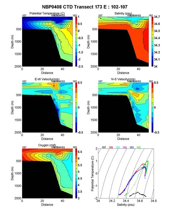
both ISW and HSSW near the shelf break at this time of year present an interesting
puzzle, one that may require more than the narrowly-focused AnSlope data sets
to solve.
1.4
Acknowledgements
1.5 AnSlope-3, Personnel
2 Program Reports
2.1 CTD
2.2 Lowered Acoustic Doppler Current Profiler
(LADCP)
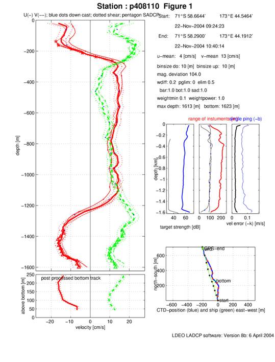
2.3 Turbulence Measurements
with “Vampire”
Deployment 3: Mixing over the Drygalski Trough sill
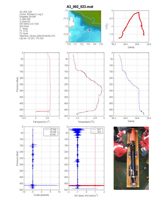
Figure 4: Example Vampire profile from Deployment 3
over the sill at the northern end of the Drygalski Trough. Location is shown
as a red dot on the map (upper center). Upper right: T-S relationship from
Seabird (CTD-quality) sensors. Middle left: profile of fall speed (m s-1).
Middle center: profiles of temperature from SeaBird SBE-3 (blue) and FP07
microstructure sensor (red), which is calibrated against the SBE-3. Middle
right: profile of salinity derived from Seabird sensors. Lower left: profile of
microscale gradient, ¶T/¶z, from FP07 thermistor. Lower center: profile of velocity shear, ¶u/¶z, from airfoil
shear probe (only shear-1 installed for this profile). Lower right: photo of
Vampire being prepared in the Baltic Room.
2.4 Salinity (Autosal) and T/C Sensor Behavior
Run
Although the drift in DeltaS values coincided with Autosal run # 19, no
problems were observed in the pre- and post-standarizations of the salinometer.
Standby readings also showed no significant change relative to prior or
subsequent runs. Finally, the rate of change in DeltaS is larger for the
primary sensor (change in DeltaS of +0.0115) than for the secondary sensor
(where change was less than +0.005), as shown in Figure 5. This differential
behavior was also observed in the salinity difference between the primary and
secondary sensors (see below). After station 140, the primary conductivity
sensor was soaked (for 15 min.) and flushed with a 1% solution of Triton X
100. No subsequent changes in the offset were observed.

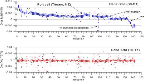
2.5 Dissolved Oxygen
Titration
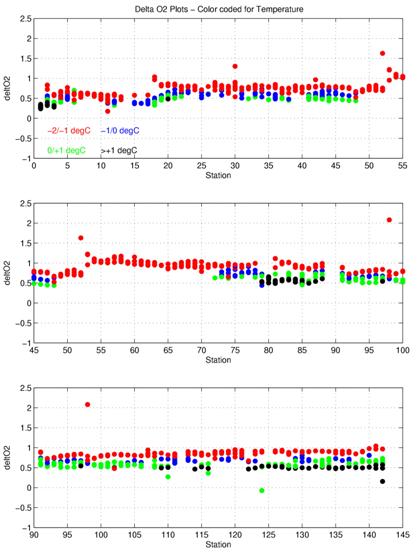
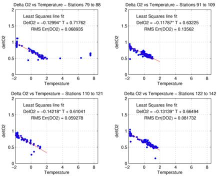
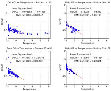
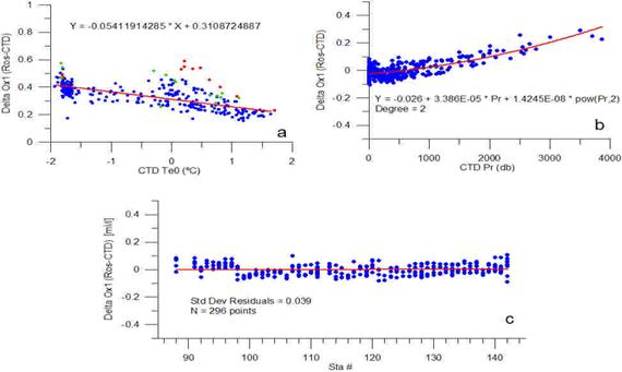
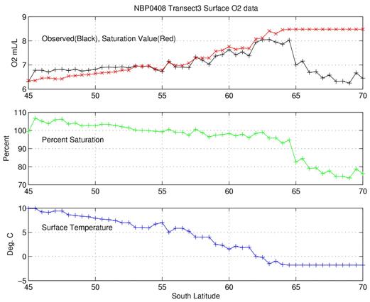
2.6 CFC-Sampling
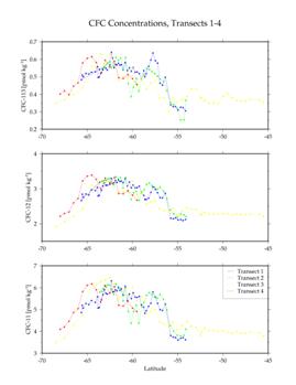
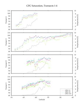
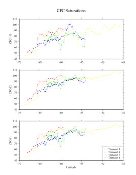
2.7 Transient Tracers (He, Tritium, O-18)
2.8 Nutrient Sampling and Analysis
 Figure 14. Temperature
and silicate concentration versus latitude in XBT section 1 (15-20 October).
Figure 14. Temperature
and silicate concentration versus latitude in XBT section 1 (15-20 October).
2.9 XBT Transit and Underway Measurements
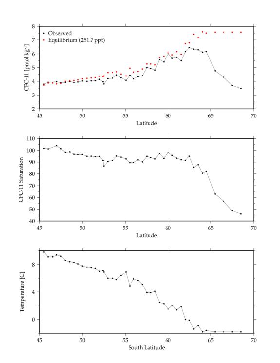
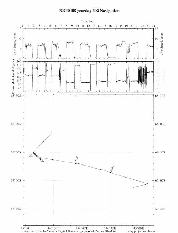
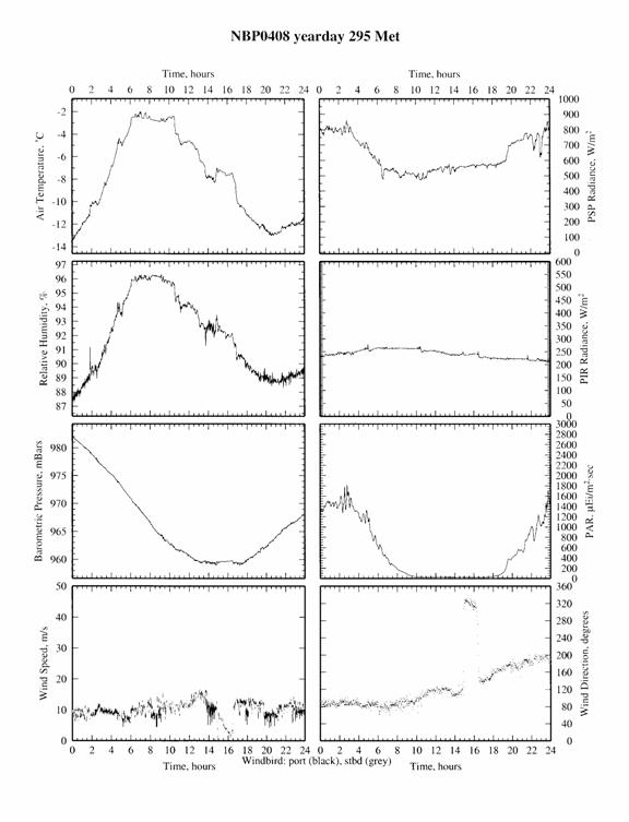
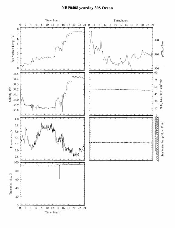

2.10 Ship-mounted ADCP Measurements (SADCP)
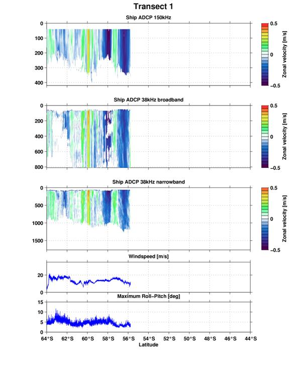
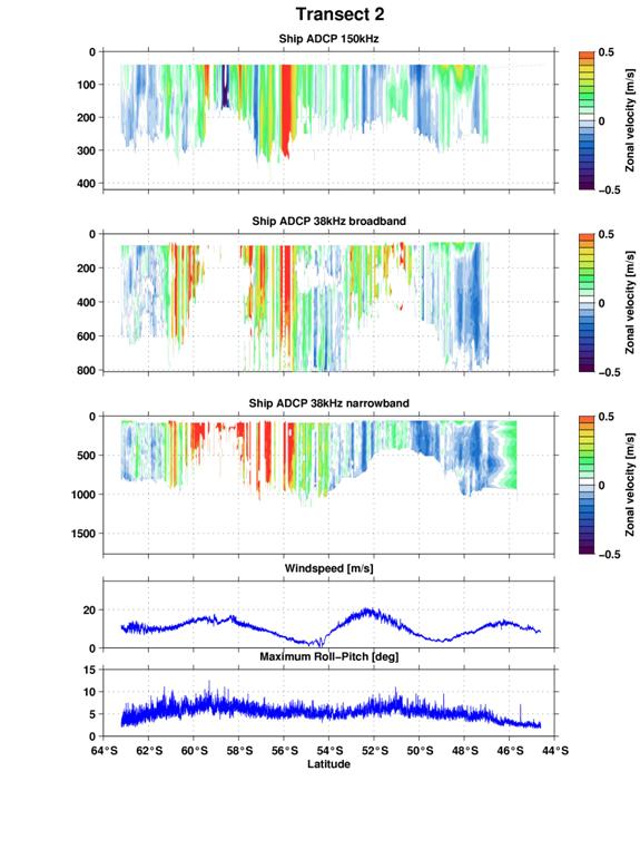
2.11 Ship acoustic systems: influence of thrusters
on on-station data quality
2.12 Oceanographic conditions in northern iceberg
field near 57.5oS
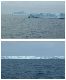 XBT
profiles taken through the field (Figure 25) confirm the reduction in SST
seen in the underway data. These profiles show the icebergs to be located in an
irregular transition zone between cooler upper-ocean (above ~300 m depth)
water to the south and warmer water north. In the profile taken within the
iceberg field (T-7#347; green), the layer of cooled, fresh water (presumably a
result of iceberg melting), is only ~20 m thick. The deeper portion of this
profile shows 3 cold intrusions, near 210, 390, and 450 m. While the origin of
these intrusions is unknown, at least the ~210 m intrusion may be the
result of lateral spreading of melt-water from the icebergs’ base.
XBT
profiles taken through the field (Figure 25) confirm the reduction in SST
seen in the underway data. These profiles show the icebergs to be located in an
irregular transition zone between cooler upper-ocean (above ~300 m depth)
water to the south and warmer water north. In the profile taken within the
iceberg field (T-7#347; green), the layer of cooled, fresh water (presumably a
result of iceberg melting), is only ~20 m thick. The deeper portion of this
profile shows 3 cold intrusions, near 210, 390, and 450 m. While the origin of
these intrusions is unknown, at least the ~210 m intrusion may be the
result of lateral spreading of melt-water from the icebergs’ base.
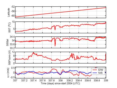
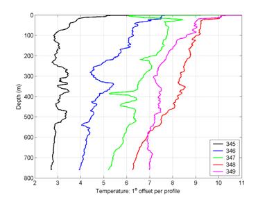
3 Station Maps and Tables
3.1 Station Maps
![Text Box: Figure A.1. CTD station locations for the first leg of Anslope-3 off the George V Coast Bathymetry from BEDMAP [Lythe et al., 2000], which is inaccurate in many locations, coastline approximate.
Lythe, M.B., Vaughan, D.G. and the BEDMAP CONSORTIUM, 2000, BEDMAP - bed topography of the Antarctic. 1:10,000,000 scale map. BAS (Misc) 9. Cambridge, British Antarctic Survey.](cruise_rep_nocontacts_filt_files/image037.gif)
3.2 CTD/LADCP Stations
3.3 NBP04-08 LADCP Profile Quality

4 Other Project Reports
4.1 Sea Ice Observations
![]()
![]()
![]()
![]() Frazil –
Grease
First year etc
Frazil –
Grease
First year etc
4.2 Marine Mammal Passive Acoustic Monitoring and
Cetacean and Wildlife Diversity
Cetacean species
Table 7: Cetacean species
sighted for the voyage NBP04-08 to 3rd December 2004.
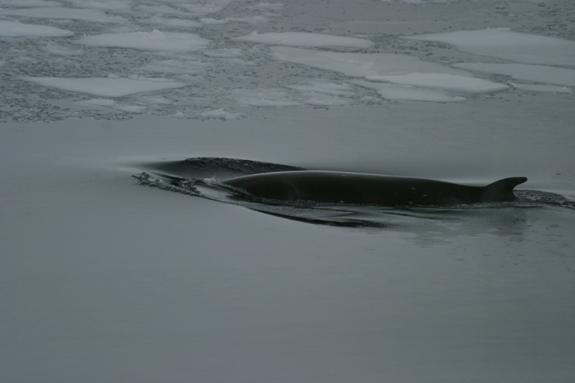
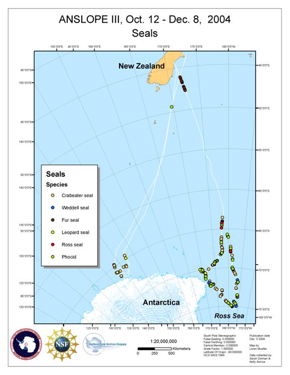
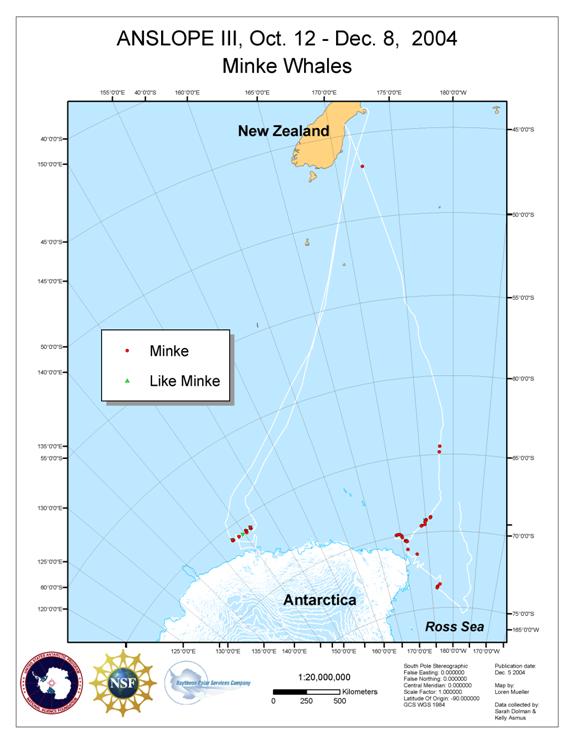
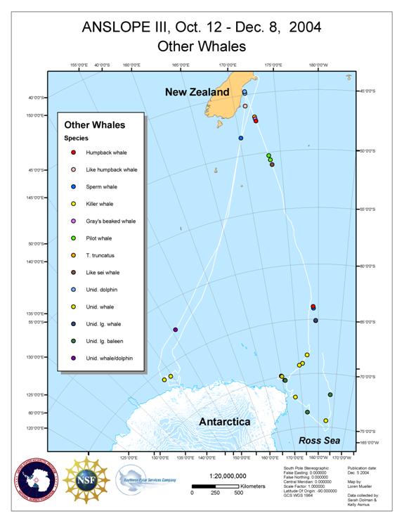
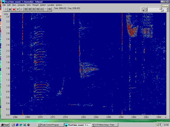
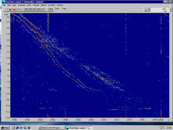
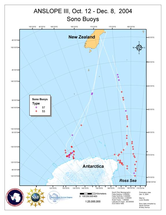
4.3 Ornithological Observations

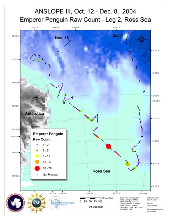
4.4 Educational/Public Outreach
4.5 Satellite Imagery
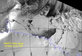
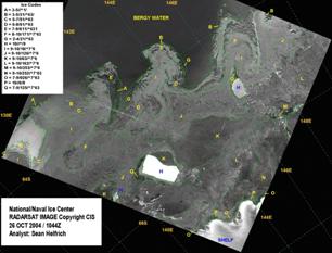
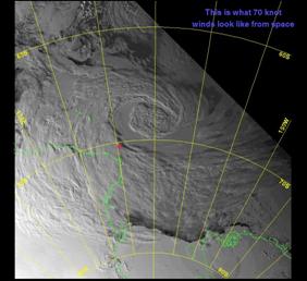
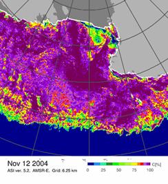
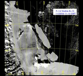
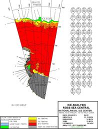
4.6 Weekly Reports
During the first leg of NBP04-08, which lasted about 25 days, about half of our
time was spent in transit to the ice edge, and roughly 1/3 of the 'in ice' time
on station, i.e., with the CTD or VMP in the water. In retrospect, the
increase in transit time on 04-08 would have provided opportunities for multibeam
work, support for which was not requested due to the anticipated 50 days in the
ice. Aside from the time in port, fuel usage during the past week has varied
from 12,200 to 5,700 gpd for SOGs of ~13.3 to 9.8 kts, both in good weather.
For those who may be interested in the continuing fuel follies saga, a brief update.
From 17 through 23 November we consumed 48,400 gallons of the precious shiply
fluids, ranging from a low of 4,000 while drifting on station to a high of
10,100 while backing and ramming through heavily ridged ice. One likely
impact of such heavy net consumption will be a reduction in the remaining
number of days that can be devoted to science, prior to our transit back to an
oil pier. An informal request for an additional 10% allowance over the official
200k gallon fuel restriction was denied by NSF. Plans are thus being
hatched to drift for a few weeks, make offerings of excess desserts to the
weather gods, and/or to expend more NBP time than necessary in LYT harbor.
I Southey and S Dolman contributed to this report. Special thanks to K Pedigo,
who bit the bullet that SeaSpace had not, tracked down the elusive Comiso
Bootstrap algorithm, wrote the script necessary to convert passive microwave
brightness temperatures to ice concentrations, and implemented same on the
ship's TeraScan. In the process, he demonstrated that one must be careful what
one asks for, since the resulting images are, for operational purposes,
inferior to Ice 85 and not substantially different from the more commonly used
'NASA Team.'
SS Jacobs